explain the difference from an standard sudden expansion case
investigate the effect of two turbulence modeling on prediction of pressure drops and velocity profiles
iterate on the methods to address convergence issues observed during the simulation
prepare the ground work required to simulate a case where the orifice is at the center of the height of the duct
To demonstrate the fact that there is no universal rule and method in CFD simulation for even simple flows like this. It is extremely important to develop an experienced-based guidelines if one is interested in accurate QUANTITATIVE results. Note that the qualitative result will still be OK and lead you to right direction.
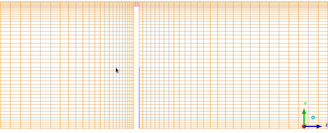
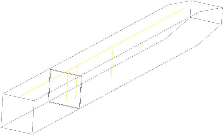
The computational domain used for this parametric study is described in following sketch. The cross-section of the duct is 70 [mm] x 70 [mm], the orifice opening is 2.5 mm and thickness of the orifice is 3.0 [mm]. The orifice is all along the width of the duct.
The boundary condition, material properties and solver setting are as per this CCL file.
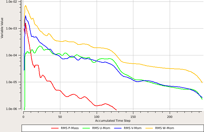
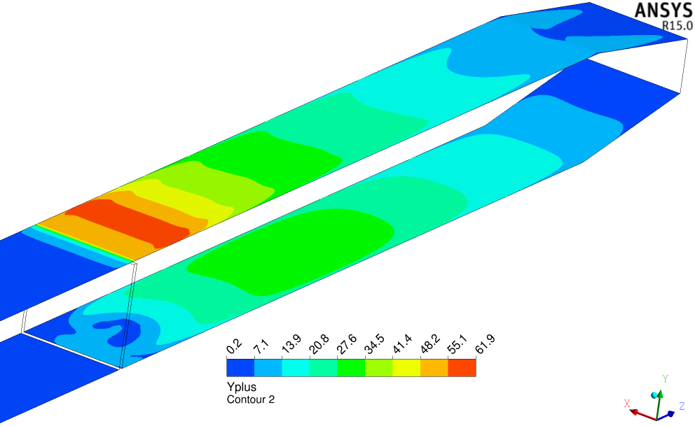
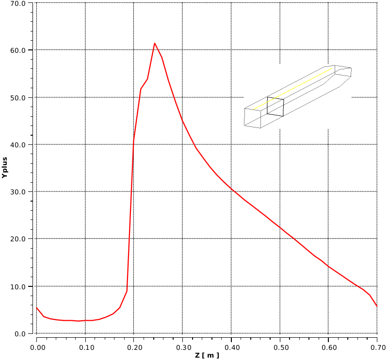
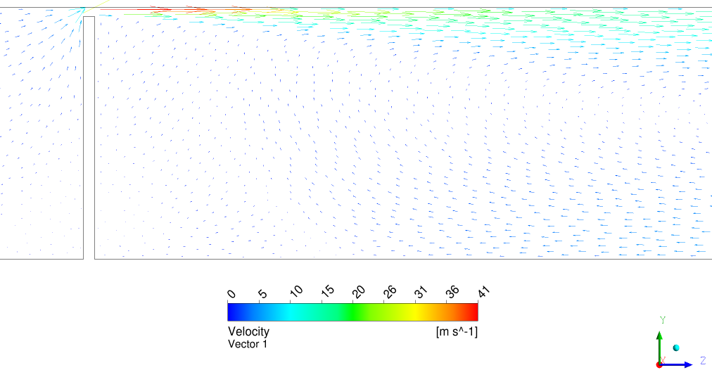
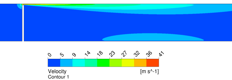
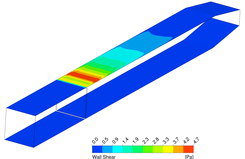
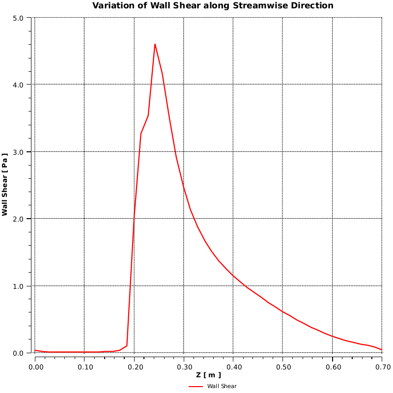
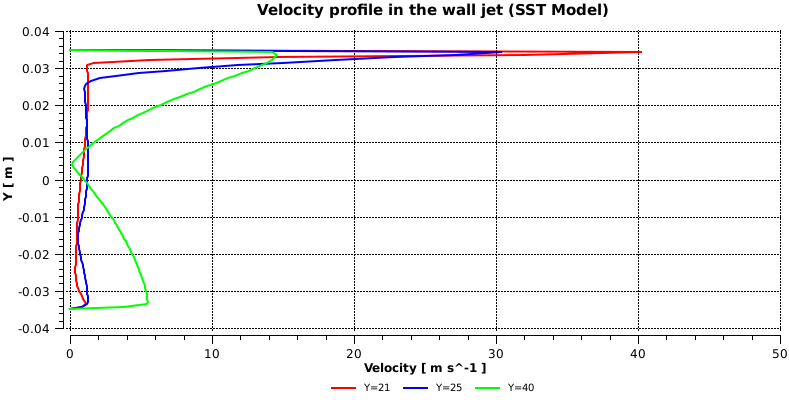
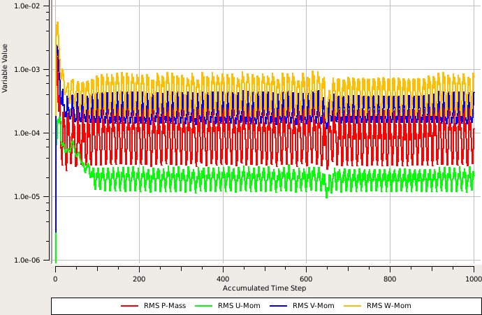
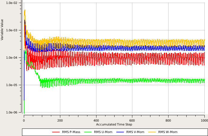
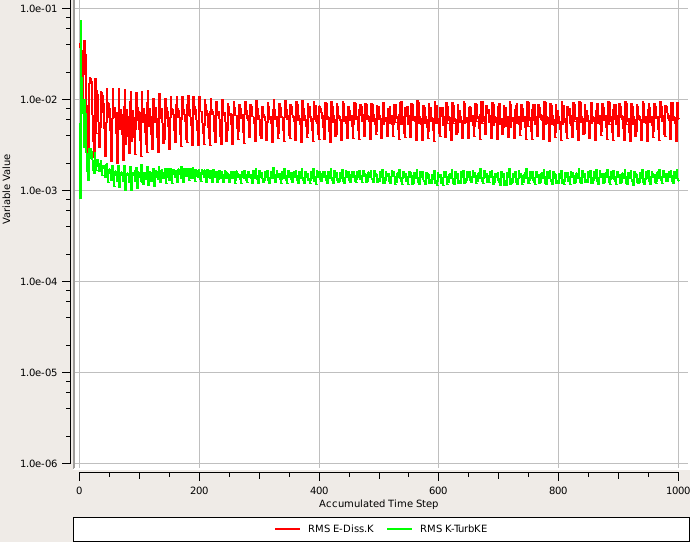
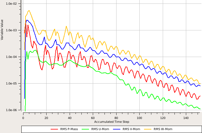
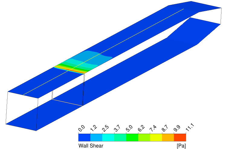
The results with Shear Stress Transport (SST) turbulence model is presented in following plots.
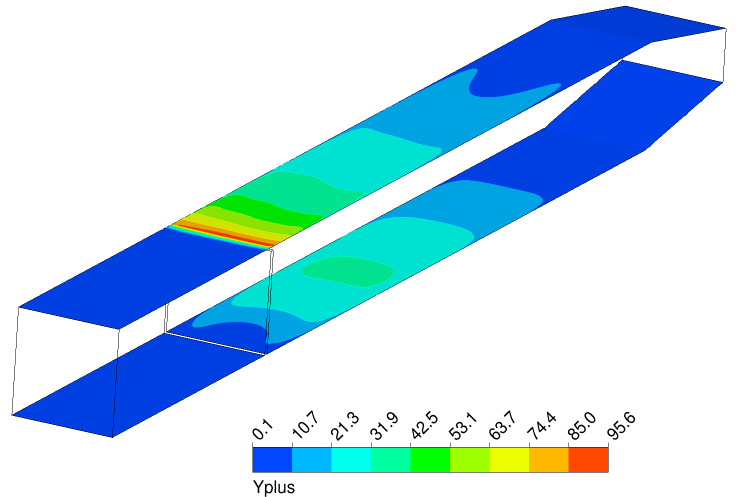
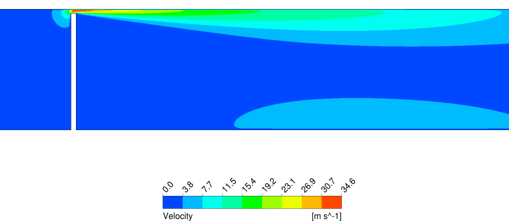
The plots Y+, velocity contour and wall shear on top wall are shown here.
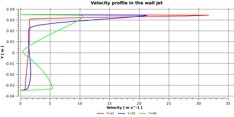
Figure: Convergence history with SST turbulence model Figure: Y-plus contour with SST turbulence model Figure: Y+ chart with SST turbulence model Figure: Velocity vector with SST turbulence model Figure: Velocity contour with SST turbulence model Figure: Wall shear stress contour with SST turbulence model Figure: Wall shear stress chart with SST turbulence model Figure: Locations for plotting velocity profile inside Wall Jet Figure: Velocity profile inside Wall Jet downstream the expansion
The results with k-ε model is presented in following plots.
Note the effect of turbulent intensity at the inlet.
The residuals show large fluctuations in case of medium (5%) and (10%) turbulent intensity. A good convergence cannot be achieved in these cases.
The residuals show fluctuations with downward bias (towards better convergence) in case of low (1%) turbulent intensity.
Figure: Convergence history with high value of turbulent intensity at inlet & k-ε model Figure: Convergence history with medium value of turbulent intensity at inlet & k-ε model Figure: Convergence history with medium value of turbulent intensity at inlet & k-ε model Figure: Convergence history with low value of turbulent intensity at inlet & k-ε model Figure: Y+ with medium value of turbulent intensity at inlet & k-ε model Figure: Velocity contour with medium value of turbulent intensity at inlet & k-ε model Figure: Wall shear with medium value of turbulent intensity at inlet & k-ε model Figure: Velocity Profile with medium value of turbulent intensity at inlet & k-ε model
Note that the Y+ value reported in k-ε model with scalable wall function is different from the one reported in SST model with automatic wall function.
The velocity in the wall jet reported by k-ε model with scalable wall function is significantly lower than the value in SST model with automatic wall function.
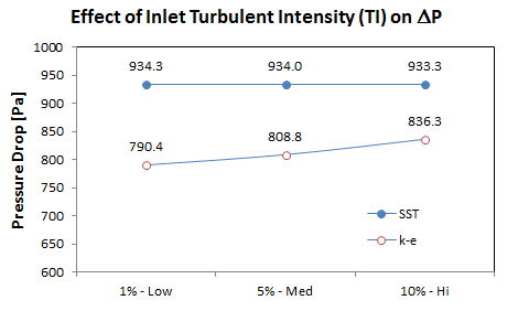
The effect of turbulent intensity on the calculated pressure drop is compared in plot below. Note that the effect of TI is less in case of SST than that in k-ε. At the same time, the reported pressure drop is significantly lower in case of k-ε model.
Figure: Effect of turbulent intensity at inlet on pressure drop in SST and k-ε model
The content on CFDyna.com is being constantly refined and improvised with on-the-job experience, testing, and training. Examples might be simplified to improve insight into the physics and basic understanding. Linked pages, articles, references, and examples are constantly reviewed to reduce errors, but we cannot warrant full correctness of all content.