- Artificial Intelligence, Machine Learning, Python, Web Scraping: Feedbacks/Queries -
Artificial Intelligence
Machine Learning Methods and Scripts
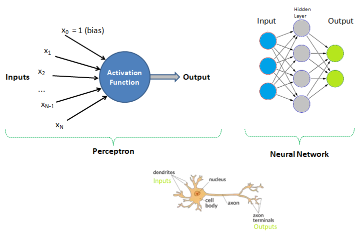
Table of Contents
- Regression and Logistic Regression (GNU OCTAVE) [*] Linear Algebra ---Principal Component Analysis (*) PCA (GNU OCTAVE) {*}K-Nearest Neighbours (KNN) using Python + sciKit-Learn --- clustering by K-means (GNU OCTAVE) ---Probability in Machine Learning
- SVM using Python + sciKit-Learn --- Naive Bayes classification --- Anomaly Detection --- Recommender Systems and Collaborative Filtering --- Decision Tree / Random Forest Classification with Python + sciKit-Learn
- Python install / update -|- OCTAVE vs. Python -|- Python Argument Parsing | Vectorization | Arrays / Slicing of Arrays || OOP in Python -|- Web Scraping in Python -|- Tuple and Dictionaries || Create Animations using Python *!* Scale all images in a folder |:| Pandas |-| File Operations in Python
- Pixels, DPI, PPI and Screen Resolution |:| Digit Recognition and ANN MLP classifications --- Computer Vision | Image Editing using ImageMagick |:| Unsharp Mask [] Image Denoising using ML |*| Rasterize and Vectorize --- Convolution, Edge Detection, Sobel kernel, Smoothen, Sharpen and Intensify Images
- Video Editing --- Image Filtering, Masking and Denoising ---Image Deskewing -|- Audio and Video Codecs | Video Editing using FFmpeg | Simple Rescaling | Create Videos from Images |:| Timeline editing and trimming |:| Crop videos | Overlay videos |:| Concatendate videos | Pillarboxing: add padding to videos |-| Color Effects |:| Freeze Effect [] Overlay videos using MoviePy --- Animations like PowerPoint |:| Box Transition Effect !! Cube Transition |=| Arrow Transition --- Animations using Blender -|- Image and Video Editing using OpenCV |+| PowerBI and Pivot Table
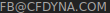
Human Brain: Have you tried to search online the keywords "number of neurons in the brain"? The answer is invariably 100 billions! There is another data that we use only 1% of brain and hence do the number 1 billion neurons not astonish you? Can we build a machine and the learning algorithm to deal with similar number of neurons?
What to Expect On This Page
Each statement is commented so that you easily connect with the code and the function of each module - remember one does not need to understand everything at the foundational level - e.g. the linear algebra behind each algorithm or optimization operations! The best way is to find a data, a working example script and fiddle with them.

✍Machine learning, artificial intelligence, cognitive computing, deep learning... are emerging and dominant conversations today all based on one fundamental truth - follow the data. In contrast to explicit (and somewhat static) programming, machine learning uses many algorithms that iteratively learn from data to improve, interpret the data and finally predict outcomes. In other words: machine learning is the science of getting computers to act without being explicitly programmed every time a new information is received.
An excerpt from Machine Learning For Dummies, IBM Limited Edition: "AI and machine learning algorithms aren't new. The field of AI dates back to the 1950s. Arthur Lee Samuels, an IBM researcher, developed one of the earliest machine learning programs - a self-learning program for playing checkers. In fact, he coined the term machine learning. His approach to machine learning was explained in a paper published in the IBM Journal of Research and Development in 1959". There are other topics of discussion such as Chinese Room Argument to question whether a program can give a computer a 'mind, 'understanding' and / or 'consciousness'. This is to check the validity of Turing test developed by Alan Turing in 1950. Turing test is used to determine whether or not computer (or machines) can think (intelligently) like humans.
The technical and business newspapers/journals are full of references to "Big Data". For business, it usually refers to the information that is capture or collected by the computer systems installed to facilitate and monitor various transactions. Online stores as well as traditional bricks-and-mortar retail stores generate wide streams of data. Big data can be and are overwhelming consisting of data table with millions of rows and hundreds if not thousands of columns. Not all transactional data are relevant though! BiG data are not just big but very often problematic too - containing missing data, information pretending to be numbers and outliers.
◎Data Management
Data management is art of getting useful information from raw data generated within the business process or collected from external sources. This is known as data science and/or data analytics and/or big data analysis. Paradoxically, the most powerful growth engine to deal with technology is the technology itself. The internet age has given data too much to handle and everybody seems to be drowning in it. Data may not always end up in useful information and a higher probability exists for it to become a distraction. Machine learning is related concept which deals with Logistic Regression, Support Vector Machines (SVM), k-Nearest-Neighbour (KNN) to name few methods.
Before one proceed further, let's try to recall how we were taught to make us what is designated as an 'educated or learned' person (we all have heard about literacy rate of a state, district and the country).
| Classical Learning Method | Example | Applicable to Machine Learning? |
| Instructions: repetition in all 3 modes - writing, visual and verbal | How alphabets and numerals look like | No |
| Rule | Counting, summation, multiplication, short-cuts, facts (divisibility rules...) | No |
| Mnemonics | Draw parallel from easy to comprehend subject to a tougher one: Principal (Main), Principle (Rule) | Yes |
| Analogy | Comparison: human metabolic system and internal combustion engines | No |
| Inductive reasoning and inferences | Algebra: sum of first n integers = n(n+1)/2, finding a next digit or alphabet in a sequence | Yes |
| Theorems | Trigonometry, coordinate geometry, calculus, linear algebra, physics, statistics | Yes |
| Memorizing (mugging) | Repeated speaking, writing, observing a phenomenon or words or sentences, meaning of proverbs | Yes |
| Logic and reasoning | What is right (appropriate) and wrong (inappropriate), interpolation, extrapolation | Yes |
| Reward and punishment | Encourage to act in a certain manner, discourage not to act in a certain manner | Yes |
| Identification, categorization and classification | Telling what is what! Can a person identify a potato if whatever he has seen in his life is the French fries? | Yes |
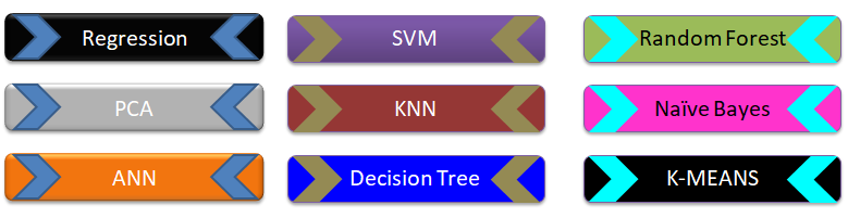
This is just a demonstration (using Python and scikit-learn) of one out of many machine learning methods which let users know what to expect as someone wants to dive deeper. One need not understand every line of the code though comments have been added to make the readers grab most out of it. The data in CSV format can be downloaded from here.
#      CLASSIFICATION: 'DECISION TREE' USING PYTHON + SCIKIT-LEARN

#On WIN10, python version 3.5
#Install scikit-learn: C:\WINDOWS\system32>py.exe -m pip install -U scikit-learn
#pip install -r list.txt - install modules (1 per line) described in 'list.txt'

# Decision Tree method is a 'supervised' classification algorithm.
# Problem Statement: The task here is to predict whether a person is likely to
# become diabetic or not based on 4 attributes: Glucose, BloodPressure, BMI, Age

# Import numPy (mathematical utility) and Pandas (data management utility)
import numpy as np
import pandas as pd
import matplotlib.pyplot as plt

# Import train_test_split function from ML utility scikit-learn for Python
from sklearn.model_selection import train_test_split

#Import scikit-learn metrics module for accuracy calculation
from sklearn import metrics

#Confusion Matrix is used to understand the trained classifier behavior over the
#input or labeled or test dataset
from sklearn.metrics import confusion_matrix
from sklearn.metrics import accuracy_score
from sklearn.metrics import classification_report

from sklearn import tree
from sklearn.tree import DecisionTreeClassifier, plot_tree
from sklearn.tree.export import export_text
# Import dataset: header=0 or header =[0,1] if top 2 rows are headers
df = pd.read_csv('diabetesRF.csv', sep=',', header='infer')

# Printing the dataset shape
print ("Dataset Length: ", len(df))
print ("Dataset Shape: ", df.shape)
print (df.columns[0:3])
# Printing the dataset observations
print ("Dataset: \n", df.head())

# Split the dataset after separating the target variable
# Feature matrix
X = df.values[:, 0:4] #Integer slicing: note columns 1 ~ 4 only (5 is excluded)
#To get columns C to E (unlike integer slicing, 'E' is included in the columns)

# Target variable (known output - note that it is a supervised algorithm)
Y = df.values[:, 4]

# Splitting the dataset into train and test
X_trn, X_tst, Y_trn, Y_tst = train_test_split(X, Y, test_size = 0.20,
    random_state = 10)
#random_state: If int, random_state is the seed used by random number generator
#print(X_tst)

#test_size: if 'float', should be between 0.0 and 1.0 and represents proportion
#of the dataset to include in the test split. If 'int', represents the absolute
#number of test samples.  If 'None',  the value is set to the complement of the
#train size. If train_size is also 'None', it will be set to 0.25.
# Perform training with giniIndex.  Gini Index is a metric to measure how often
# a randomly chosen element would be incorrectly identified (analogous to false
# positive and false negative outcomes).

# First step: #Create Decision Tree classifier object named clf_gini
clf_gini = DecisionTreeClassifier(criterion = "gini", random_state=100,
    max_leaf_nodes=3, max_depth=None, min_samples_leaf=3)

#'max_leaf_nodes': Grow a tree with max_leaf_nodes in best-first fashion. Best
#nodes are defined as relative reduction in impurity. If 'None' then unlimited
#number of leaf nodes.

#max_depth = maximum depth of the tree. If None, then nodes are expanded until
#all leaves are pure or until all leaves contain < min_samples_split samples.

#min_samples_leaf = minimum number of samples required to be at a leaf node. A
#split point at any depth will only be considered if it leaves at least
#min_samples_leaf training samples in each of the left and right branches.

# Second step: train the model (fit training data) and create model gini_clf
gini_clf = clf_gini.fit(X_trn, Y_trn)

# Perform training with entropy, a measure of uncertainty of a random variable.
# It characterizes the impurity of an arbitrary collection of examples. The
# higher the entropy the more the information content.
clf_entropy = DecisionTreeClassifier(criterion="entropy", random_state=100,
    max_depth=3, min_samples_leaf=5)
entropy_clf = clf_entropy.fit(X_trn, Y_trn)
# Make predictions with criteria as giniIndex or entropy and calculate accuracy
Y_prd = clf_gini.predict(X_tst)

#y_pred = clf_entropy.predict(X_tst)

#-------Print predicted value for debugging purposes ---------------------------
#print("Predicted values:")
#print(Y_prd)

print("Confusion Matrix for BINARY classification as per sciKit-Learn")
print("    TN   |    FP   ")
print("-------------------")
print("    FN   |    TP   ")
print(confusion_matrix(Y_tst, Y_prd))

# Print accuracy of the classification = [TP + TN] / [TP+TN+FP+FN]
print("Accuracy = {0:8.2f}".format(accuracy_score(Y_tst, Y_prd)*100))

print("Classification Report format for BINARY classifications")
#                           P           R           F           S
#                       Precision     Recall      fl-Score    Support
#       Negatives (0)   TN/[TN+FN]    TN/[TN+FP]  2RP/[R+P]   size-0 = TN + FP
#       Positives (1)   TP/[TP+FP]    TP/[TP+FN]  2RP/[R+P]   size-1 = FN + TP
# F-Score = harmonic mean of precision and recall - also known as the Sorensen–
# Dice coefficient or Dice similarity coefficient (DSC).
# Support = class support size (number of elements in each class).
print("Report: ", classification_report(Y_tst, Y_prd))

''' ---- some warning messages -------------- ------------- ---------- ----------
Undefined Metric Warning: Precision and F-score are ill-defined and being set to
0.0 in labels with no predicted samples.
- Method used to get the F score is from the "Classification" part of sklearn
- thus it is talking about "labels".  This means that there is no "F-score" to
calculate for some label(s) and F-score for this case is considered to be 0.0.
'''

#from matplotlib.pyplot import figure
#figure(num=None, figsize=(11, 8), dpi=80, facecolor='w', edgecolor='k')
#figure(figsize=(1,1)) would create an 1x1 in image = 80x80 pixels as per given
#dpi argument.

plt.figure()
fig = plt.gcf()
fig.set_size_inches(15, 10)

clf = DecisionTreeClassifier().fit(X_tst, Y_tst)
plot_tree(clf, filled=True)

fig.savefig('./decisionTreeGraph.png', dpi=100)
#plt.show()
#---------------------- ------------------------ ----------------- ------------
#Alternate method to plot the decision tree is to use GraphViz module
#Install graphviz in Pyhton- C:\WINDOWS\system32>py.exe -m pip install graphviz
#Install graphviz in Anaconda: conda install -c conda-forge python-graphviz
#---------------------- ------------------------ ----------------- ------------
Data management is the method and technology of getting useful information from raw data generated within the business process or collected from external sources. Have you noticed that when you search for a book-shelf or school-shoes for your kid on Amazon, you start getting google-ads related to these products when you browse any other website? Your browsing history is being tracked and being exploited to remind you that you were planning to purchase a particular type of product! How is this done? Is this right or wrong? How long shall I get such 'relevant' ads? Will I get these ads even after I have already made the purchase?
The answer to all these questions lies in the way "data analytics" system has been designed and the extent to which it can access user information. For example, are such system allowed to track credit card purchase frequency and amount?
Related fields are data science, big data analytics or simply data analytics. 'Data' is the 'Oil' of 21st century and machine learning is the 'electricity'! This is a theme floating around in every organization, be it a new or a century old well-established company. Hence, a proper "management of life-cycle" of the data is as important as any other activities necessary for the smooth functioning of the organization. When we say 'life-cycle', we mean the 'generation', 'classification', "storage and distribution", "interpretation and decision making" and finally marking them 'obsolete'.
Due to sheer importance and size of such activities, there are many themes such as "Big Data Analytics". However, the organizations need not jump directly to a large scale analytics unless they test and validate a "small data analytics" to develop a robust and simple method of data collection system and processes which later complements the "Big Data Analytics". We also rely on smaller databases using tools which users are most comfortable with such as MS-Excel. This helps expedite the learning curve and sometimes even no new learning is required to get started.

Before proceeding further, let's go back to the basic. What do we really mean by the word 'data'? How is it different from words such as 'information' and 'report'? Data or a dataset is a collection of numbers, labels and symbols along with context of those values. For the information in a dataset to be relevant, one must know the context of the numbers and text it holds. Data is summarized in a table consisting of rows (horizontal entries) and columns (vertical entries). The rows are often called observations or cases.
Columns in a data table are called variables as different values are recorded in same column. Thus, columns of a dataset or data table describes the common attribute shared by the items or observations.
Let's understand the meaning and difference using an example. Suppose you received an e-mail from your manager requesting for a 'data' on certain topic. What is your common reply? Is it "Please find attached the data!" or is it "Please find attached the report for your kind information!"? Very likely the later one! Here the author is trying to convey the message that I have 'read', 'interpreted' and 'summarized' the 'data' and produced a 'report or document' containing short and actionable 'information'.
The 'data' is a category for 'information' useful for a particular situation and purpose. No 'information' is either "the most relevant" or "the most irrelevant" in absolute sense. It is the information seeker who defines the importance of any piece of information and then it becomes 'data'. The representation of data in a human-friendly manner is called 'reporting'. At the same time, there is neither any unique way of extracting useful information nor any unique information that can be extracted from a given set of data. Data analytics can be applied to any field of the universe encompassing behaviour of voters, correlation between number of car parking tickets issued on sales volume, daily / weekly trade data on projected movement of stock price...
Types of Documents
| Structured | Semi-Structured | Unstructured |
| The texts, fonts and overall layout remains fixed | The texts, fonts and overall layout varies but have some internal structure | The texts, fonts and overall layout are randomly distributed |
| Examples are application forms such as Tax Return, Insurance Policies | Examples are Invoices, Medical est reports | E-mails, Reports, Theses, Sign-boards, Product Labels |
Computers understand data in a certain format whereas the nature of data can be numbers as well as words or phrases which cannot be quantified. For example, the difference in "positive and neutral" ratings cannot be quantified and will not be same as difference in "neutral and negative" ratings. There are many ways to describe the type of data we encounter in daily life such as (binary: either 0 or 1), ordered list (e.g. roll number or grade)...
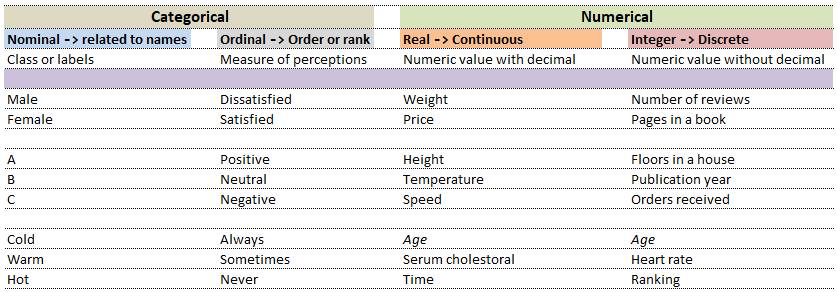
| Nominal | Ordinal | ||
| What is your preferred mode of travel? | How will you rate our services? | ||
| 1 | Flights | 1 | Satisfied |
| 2 | Trains | 2 | Neutral |
| 3 | Drive | 3 | Dissatisfied |
While in the first case, digits 1, 2 and 3 are just variable labels [nominal scale] whereas in the second example, the same numbers (digits) indicate an order [ordinal scale]. Similarly, phone numbers and pin (zip) codes are 'numbers' but they form categorical variables as no mathematical operations normally performed on 'numbers' are applicable to them.

Data Analytics, Data Science, Machine Learning, Artificial Intelligence, Neural Network and Deep Learning are some of the specialized applications dealing with data. There is no well-defined boundaries as they necessarily overlap and the technology itself is evolving at rapid pace. Among these themes, Artificial Neural Network (ANN) is a technology inspired by neurons in human brains and ANN is the technology behind artificial intelligence where attempts are being made to copy how human brain works. 'Data' in itself may not have 'desired' or 'expected' value and the user of the data need to find 'features' to make machine learning algorithms works as most of them expect numerical feature vectors with a fixed size. This is also known as "feature engineering".
- Artificial Intelligence (AI): Self-driving car (autonomous vehicles), speech recognition
- Machine Learning (ML): Given a picture - identify steering angle of a car, Google translate, Face recognition, Identify hand-written letters.
| Artificial Intelligence | Machine Learning | Deep Learning |
| Engineer | Researcher | Scientist |
| B. Tech. degree | Master's degree | PhD |
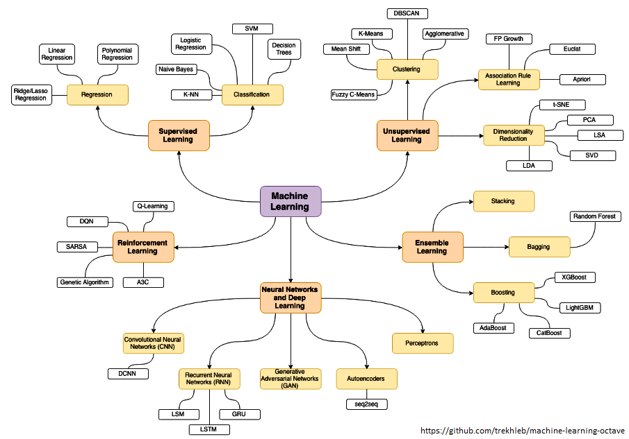
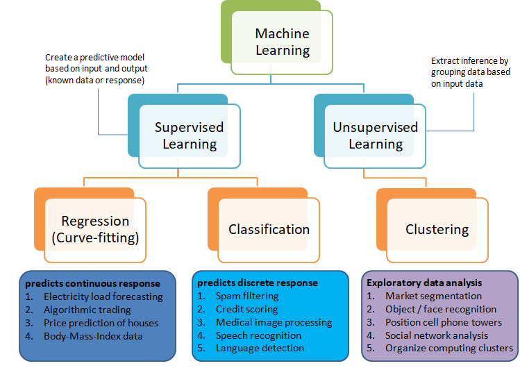
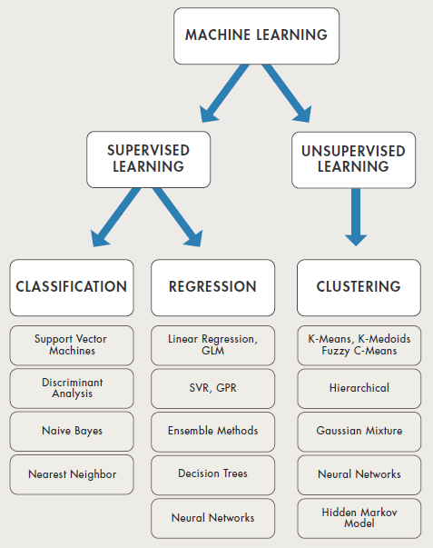
The category of supervised and unsupervised learning can be demonstrated as per the chart below. The example applications of each type of the machine learning method helps find a clear distinction among those methods. The methods are nothing new and we do it very often in our daily life. For example, ratings in terms of [poor, average, good, excellent] or [hot, warm, cold] or [below expectations, meets expectations, exceeds expectations, substantially exceeds expectations] can be based on different numerical values. Refer the customer loyalty rating (also known as Net Promoters Score) where a rating below 7 on scale of 10 is considered 'detractors', score between '7 - 8' is rated 'passive' and score only above 8 is considered 'promoter'. This highlights the fact that no uniform scale is needed for classifications.
Selection of machine learning algorithms: reference e-book "Introducing Machine Learning" by MathWorks.
Machine learning is all about data and data is all about row and column vectors. Each instance of a data or observation is usually represented by a row vector where the first or the last element may be the 'variable or category desired to be predicted'. Thus, there are two broad division of a data set: features and labels (as well as levels of the labels).
- Features: This refers to key characteristics of a dataset or entity. In other words, features are properties that describe each instance of data. Each instance is a point in feature space. For example, a car may have color, type (compact, sedan, SUV), drive-type (AWD, 4WD, FWD, RWD) ... This is also known as predictors, inputs or attributes.
- Label: This is the final identifier such as price category of a car. It is also known as the target, response or output of a feature vector.
As in any textbook, there are solved examples to demonstrate the theory explained in words, equations and figures. And then there are examples (with or without known answers) to readers to solve and check their learnings. The two sets of question can be classified as "training questions" and "evaluation questions" respectively. Similarly in machine learning, we may have a group of datasets where output or label is known and another datasets where labels may not be known.
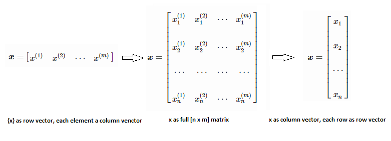
Training set is an input data where for every predefined set of features 'xi' we have a correct classification y. It is represented as tuples [(x1, y1), (x2, y2), (x3, y3) ... (xk, yk)] which represents 'k' rows in the dataset. Rows of 'x' correspond to observations and columns correspond to variables or attributes or labels. In other words, feature vector 'x' can be represented in matrix notation as: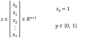
Hypothesis (the Machine Learning Model)
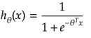
It is equation that gets features and parameters as an input and predicts the value as an output (i.e. predict if the email is spam or not based on some email characteristics). hθ(x) = g(θTx) where 'T' refers to transpose operation, θ are the (unknown) parameters evaluated during the learning process and 'g' is the Sigmoid function g(u) = [1+e-u]-1 which is plotted below.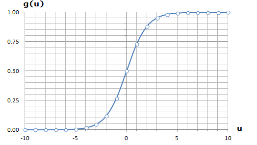
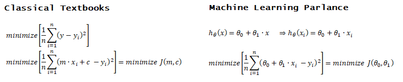
Activation Function: The hypothesis for a linear regression can be in the form y = m·x + c or y = a + b·log(c·x). The objective function is to estimate value of 'm' and 'c' by minimizing the square error as described in cost function.
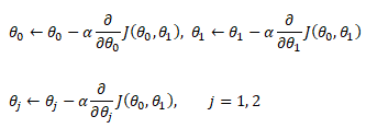
The objective function of a logistic regression can be described as:- Predict y = 0 if hθ(x) < 0.5 which is true if θTx ≥ 0.
- Predict y = 1 if hθ(x) > 0.5 which is true if θTx < 0. θi are called parameters of the model.
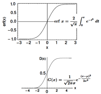
Note that the Sigmoid function looks similar to classical error function and cumulative normal distribution function with mean zero.
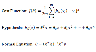
Linear regression: cost function also known as "square error function" is expressed as
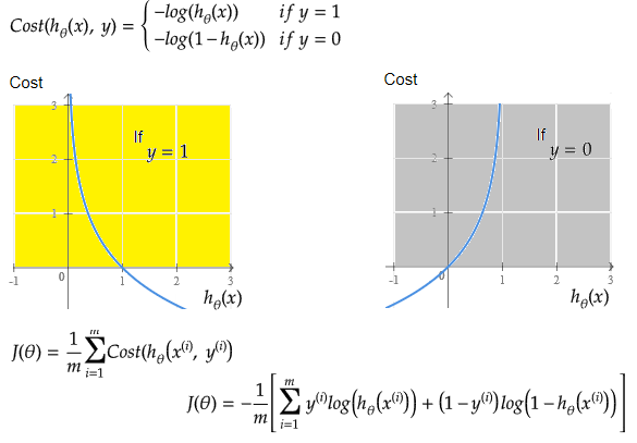
Cost(θ) = - y × log[hθ(x)] - (1-y) × [1 - log(hθ(x))]
In other words: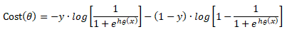
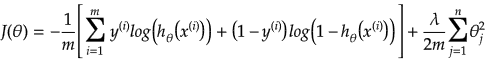
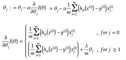
Additional method adopted is the "mean normalization" where all the features are displacement such that their means are closer to 0. These two scaling of the features make the gradient descent method faster and ensures convergence.
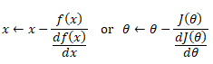
Normal Equation
This refers to the analytical method to solver for θ. If the matrix XTX is invertible, θ = (XTX)-1XTy where y is column vector of known labels (n × 1). X is features matrix of size n × (m+1) having 'n' number of datasets (rows) in training set and 'm' number of attributes.If [X] contains any redundant feature (a feature which is dependent on other features), it is likely to be XTX non-invertible.
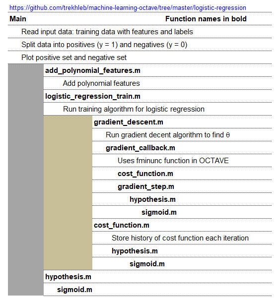
An implementation of logistic regression in OCTAVE is available on the web. One of these available in GitHub follow the structure shown below.
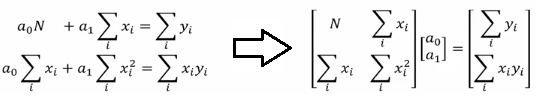
Optimization and regression using Octave - click to get the GNU OCTAVE scripts. Linear Least Square (LSS) is a way to estimate the curve-fit parameters. A linear regression is fitting a straight line y = a0 + a1x where {x} is the independent variable and y is the dependent variable. Since there are two unknowns a0 and a1, we need two equations to solve for them. If there are N data points:
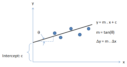
Similarly, if dependent variable y is function of more than 1 independent variables, it is called multi-variable linear regression where y = f(x1, x2...xn). The curve fit equations is written as y = a0 + a1x1 + a2x2 + ... + anxn + ε where ε is the curve-fit error. Here xp can be any higher order value of xjk and/or interaction term (xi xj).
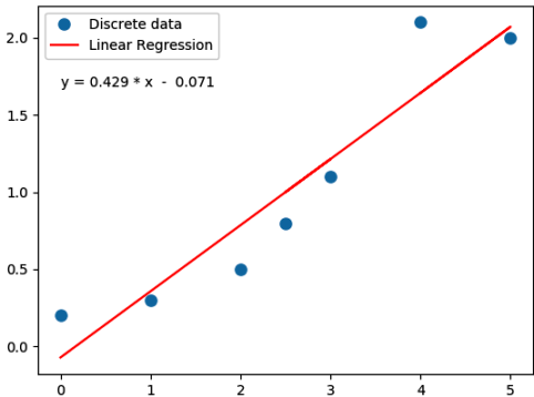
Following Python script performs linear regression and plots the discrete data, linear equation from curve-fitting operation and annotates the linear equation on the plot.
import numpy as np
#Specify coefficient matrix: independent variable values
x = np.array([0.0, 1.0, 2.0, 3.0, 2.5, 5.0, 4.0])

#Specify ordinate or "dependent variable" values
y = np.array([0.2, 0.3, 0.5, 1.1, 0.8, 2.0, 2.1])

#Create coefficient matrix
A = np.vstack([x, np.ones(len(x))]).T

#least square regression: rcond = cut-off ratio for small singular values of a
#Solves the equation [A]{x} = {b} by computing a vector x that minimizes the
#squared Euclidean 2-norm | b - {A}.{x}|^2
m, c = np.linalg.lstsq(A, y, rcond=None)[0]

print("\n Slope = {0:8.3f}".format(m))
print("\n Intercept = {0:8.3f}".format(c))

import matplotlib.pyplot as plt
_ = plt.plot(x, y, 'o', label='Discrete data', markersize=8)
_ = plt.plot(x, m*x + c, 'r', label='Linear Regression')
_ = plt.legend()
if (c > 0):
    eqn = "y ="+str("{0:6.3f}".format(m))+' * x  + '+str("{0:6.3f}".format(c))
else:
    eqn = "y ="+str("{0:6.3f}".format(m))+' * x  - '+str("{0:6.3f}".format(abs(c)))

print('\n', eqn)
#Write equation on the plot
# text is right-aligned
plt.text(min(x)*1.2, max(y)*0.8, eqn, horizontalalignment='left')
plt.show()
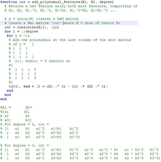
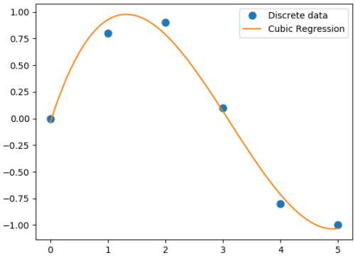
If the equation used to fit has exponent of x > 1, it is called a polynomical regression. A quadratic regression uses polynomial of degree 2 (y = a0 + a1x + a2x2 + ε), a cubic regression uses polynomial of degree 3 (y = a0 + a1x + a2x2 + a3x3 + ε) and so on. Since the coefficients are constant, a polynomial regression in one variable can be deemed a multi-variable linear regression where x1 = x, x2 = x2, x3 = x3 ... In scikit-learn, PolynomialFeatures(degree = N, interaction_only = False, include_bias = True, order = 'C') generates a new feature matrix consisting of all polynomial combinations of the features with degree less than or equal to the specified degree 'N'. E.g. poly = PolynomialFeatures(degree=2), Xp = poly.fit_transform(X, y) will transform [x1, x2] to [1, x1, x2, x1*x1, x1*x2, x2*x2]. Argument option "interaction_only = True" can be used to create only the interaction terms. Bias column (added as first column) is the feature in which all polynomial powers are zero (i.e. a column of ones - acts as an intercept term in a linear model).
Polynomial regression in single variable - Uni-Variate Polynomial Regression: The Polynomial Regression can be perform using two different methods: the normal equation and gradient descent. The normal equation method uses the closed form solution to linear regression and requires matrix inversion which may not require iterative computations or feature scaling. Gradient descent is an iterative approach that increments theta according to the direction of the gradient (slope) of the cost function and requires initial guess as well.
#Least squares polynomial fit: N = degree of the polynomial

#Returns a vector of coefficients that minimises the squared error in the order
#N, N-1, N-2 … 0. Thus, the last coefficient is the constant term, and the first
#coefficient is the multiplier to the highest degree term, x^N

import warnings; import numpy as np
x = np.array([0.0, 1.0, 2.0, 3.0,  4.0,  5.0])
y = np.array([0.0, 0.8, 0.9, 0.1, -0.8, -1.0])
#
N = 3
#full=True: diagnostic information from SVD is also returned
coeff = np.polyfit(x, y, N, rcond=None, full=True, w=None, cov=False)

np.set_printoptions(formatter={'float': '{: 8.4f}'.format})
print("Coefficients: ", coeff[0])
print("Residuals:", coeff[1])
print("Rank:", coeff[2])
print("Singular Values:", coeff[3])
print("Condition number of the fit: {0:8.2e}".format(coeff[4]))

#poly1D: A 1D polynomial class  e.g. p = np.poly1d([3, 5, 8]) = 3x^2 + 5x + 8
p = np.poly1d(coeff[0])

xp = np.linspace(x.min(), x.max(),100)
import matplotlib.pyplot as plt
_ = plt.plot(x, y, 'o', label='Discrete data', markersize=8)
_ = plt.plot(xp, p(xp), '-', label='Cubic Regression', markevery=10)
_ = plt.legend()

plt.rcParams['path.simplify'] = True
plt.rcParams['path.simplify_threshold'] = 0.0
plt.show()
Output from the above code is:
Coefficients:  [0.0870  -0.8135   1.6931  -0.0397]
Residuals: [ 0.0397]
Rank: 4
Singular Values: [1.8829   0.6471   0.1878   0.0271]
Condition number of the fit: 1.33e-15
In addition to 'poly1d' to estimate a polynomial, 'polyval' and 'polyvalm' can be used to evaluate a polynomial at a given x and in the matrix sense respectively. ppval(pp, xi) evaluate the piecewise polynomial structure 'pp' at the points 'xi' where 'pp' can be thought as short form of piecewise polynomial.
Similarly, a non-linear regression in exponential functions such as y = c × ekx can be converted into a linear regression with semi-log transformation such as ln(y) = ln(c) + k.x. It is called semi-log transformation as log function is effectively applied only to dependent variable. A non-linear regression in power functions such as y = c × xk can be converted into a linear regression with log-log transformation such as ln(y) = ln(c) + k.ln(x). It is called log-log transformation as log function is applied to both the independent and dependent variables.
A general second order model is expressed as described below. Note the variable 'k' has different meaning as compared to the one described in previous paragraph. Here k is total number of independent variables and n is number of rows (data in the dataset).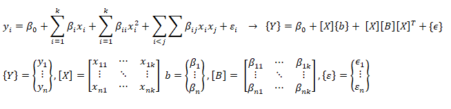
As per MathWorks: "The multivariate linear regression model is distinct from the multiple linear regression model, which models a univariate continuous response as a linear combination of exogenous terms plus an independent and identically distributed error term." Note that endogenous and exogenous variables are similar but not same as dependent and independent variables. For example, the curve fit coefficients of a linear regression are variable (since they are based on x and y), they are called endogenous variables - values that are determined by other variables in the system. An exogenous variable is a variable that is not affected by other variables in the system. In contrast, an endogenous variable is one that is influenced by other factors in the system. Here the 'system' may refer to the "regression algorithm".
In summary, categorization of regression types: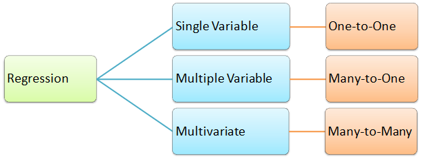
#----------------------- -------------------------- ---------------------------
import numpy as np
import pandas as pd

df = pd.read_csv('MultiVariate2.csv', sep=',', header='infer')
X = df.values[0:20, 0:3]
y = df.values[0:20, 3]

#Y = a1x1 + a2x2 + a3x3 + ... + +aNxN + c

#-------- Method-1: linalg.lstsq ---------------------- -----------------------
X = np.c_[X, np.ones(X.shape[0])] # add bias term
beta_hat = np.linalg.lstsq(X, y, rcond=None)[0]
print(beta_hat)

print("\n------ Runnning Stats Model ----------------- --------\n")
#Ordinary Least Squares (OLS), Install: py -m pip -U statsmodels
from statsmodels.api import OLS
model = OLS(y, X)
result = model.fit()
print (result.summary())

#-------- Method-3: linalg.lstsq ----------------------- ----------------------
print("\n-------Runnning Linear Regression in sklearn ---------\n")
from sklearn.linear_model import LinearRegression
regressor = LinearRegression()
regressor.fit(X, y)
print(regressor.coef_)       #print curve-fit coefficients
print(regressor.intercept_)  #print intercept values
#
#print regression accuracy: coefficient of determination R^2 = (1 - u/v), where
#u is the residual sum of squares and v is the total sum of squares.
print(regressor.score(X, y))
#
#calculate y at given x_i
print(regressor.predict(np.array([[3, 5]])))
More example of curve-fit using SciPy
'''
Curve fit in more than 1 independent variables.
Ref: stackoverflow.com/.../fitting-multivariate-curve-fit-in-python
'''
import numpy as np
import matplotlib.pyplot as plt
from scipy.optimize import curve_fit

def fit_circle(x, a, b):
  '''
  Model Function that provides the type of fit y = f(x). It must take
  the independent variable as the first argument and the parameters
  to fit as separate remaining arguments.
  '''
  return  a*x[0]*x[0] + b*x[1]*x[1]

def fit_poly(x, a, b, c, d, e, f):
  '''
  Model Function that provides the type of fit y = f(x). It must take
  the independent variable as the first argument and the parameters
  to fit as separate remaining arguments.
  '''
  return  a*x[0]*x[0] + b*x[1]*x[1] + c*x[0]*x[1] + d * x[0] + e * x[1] + f

def fit_lin_cross(x, a, b, c, d):
  '''
  Model Function that provides the type of fit y = f(x). It must take
  the independent variable as the first argument and the parameters
  to fit as separate remaining arguments.
  '''
  return a*x[0] + b*x[1] + c*x[0]*x[1] + d

def fit_2d_data(fit_func, x_data, y_data, p0=None):
  '''
  Main function to calculate coefficients.
  x_data: (k,M)-shaped array for functions with k predictors (data points)
  y_data: The dependent data, a length M array
  p0: Initial guess for the parameters (length N), default = 1
  '''
  fitParams, fitCovariances = curve_fit(fit_func, x_data, y_data, p0)

  print('Curve-fit coefficients: \n', fitParams)

# Run curve-fit. x, y and z arrays can be read from a text file.
x = np.array([1, 2, 3, 4, 5, 6])
y = np.array([2, 3, 4, 5, 6, 8])
z = np.array([5, 13, 25, 41, 61, 100])
x_data = (x, y)
fit_2d_data(fit_lin_cross, x_data, z)
Ridge Regression
If data suffers from multicollinearity (independent variables are highly correlated), the least squares estimates result in large variances which deviates the observed value far from the true value (low R-squared, R2). By adding a degree of bias to the regression estimates using a "regularization or shrinkage parameter", ridge regression reduces the standard errors. In scikit-learn, it is invoked by "from sklearn.linear_model import Ridge". The function is used by: reg = Ridge(alpha=0.1, fit_intercept=True, normalize=False, solver='auto', random_state=None); reg.fit(X_trn, y_trn). Regularization improves the conditioning of the problem and reduces the variance of the estimates. Larger values specify stronger regularization.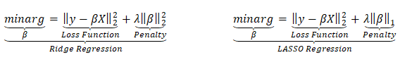
Lasso Regression
Lasso (Least Absolute Shrinkage and Selection Operator) is similar to ridge regression which penalizes the absolute size of the regression coefficients instead of squares in the later. Thus, ridge regression uses L2-regularization whereas as LASSO use L1-regularization. In scikit-learn, it is invoked by "from sklearn.linear_model import Lasso". The function is used by: reg = Lasso(); reg.fit(X_trn, y_trn)SVR
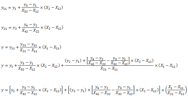
Support Vector Machines (SVM) used for classification can be extended to solve regression problems and method is called Support Vector Regression (SVR).Regression in two variables: example
| X1 | X2 | y | X1 | X2 | y | X1 | X2 | y | X1 | X2 | y | |||
| 5 | 20 | 100.0 | First Interpolation on X2 | Second Interpolation on X2 | Final interpolation on X1 | |||||||||
| 10 | 20 | 120.0 | 5 | 20 | 100.0 | 10 | 20 | 120.0 | 5 | 25 | 200.0 | |||
| 5 | 40 | 500.0 | 5 | 40 | 500.0 | 10 | 40 | 750.0 | 10 | 25 | 277.5 | |||
| 10 | 40 | 750.0 | ||||||||||||
| 8 | 25 | ? | 5 | 25 | 200.0 | 10 | 25 | 277.5 | 8 | 25 | 246.5 | |||
Interpolate your values:
| Description | Xi1 | Xi2 | yi |
| First set: | |||
| Second set: | |||
| Third set: | |||
| Fourth set: | |||
| Desired interpolation point: | |||
from sklearn.preprocessing import PolynomialFeatures
from sklearn.linear_model import LinearRegression
from sklearn import linear_model
import numpy as np
import pandas as pd
import sys
#Degree of polynomial: note N = 1 implies linear regression
N = 3;
#--------------- DATA SET-1 -------------------- ------------------- -----------
X = np.array([[0.4, 0.6, 0.8], [0.5, 0.3, 0.2], [0.2, 0.9, 0.7]])
y = [10.1, 20.2, 15.5]
print(np.c_[X, y]) # Column based concatenation of X and y arrays

#-------------- DATA SET-2 -------------- ------------------- ------------------
# Function importing Dataset
df = pd.read_csv('Data.csv', sep=',', header='infer')
#Get size of the dataframe. Note that it excludes header rows
iR, iC = df.shape

# Feature matrix
nCol = 5   #Specify if not all columns of input dataset to be considered
X = df.values[:, 0:nCol]
y = df.values[:, iC-1]
print(df.columns.values[0]) #Get names of the features

#Print header: check difference between df.iloc[[0]], df.iloc[0], df.iloc[[0,1]]
#print("Header row\n", df.iloc[0])

p_reg = PolynomialFeatures(degree = N, interaction_only=False, include_bias=False)
X_poly = p_reg.fit_transform(X)
#X will transformed from [x1, x2] to [1, x1, x2, x1*x1, x1x2, x2*x2]
X_poly = p_reg.fit_transform(X)

#One may remove specific polynomial orders, e.g. 'x' component
#Xp = np.delete(Xp, (1), axis = 1)

#Generate the regression object
lin_reg = LinearRegression()

#Perform the actual regression operation: 'fit'
reg_model = lin_reg.fit(X_poly, y)

#Calculate the accuracy
np.set_printoptions(formatter={'float': '{: 6.3e}'.format})
reg_score = reg_model.score(X_poly, y)
print("\nRegression Accuracy = {0:6.2f}".format(reg_score))
#reg_model.coef_[0] corresponds to 'feature-1', reg_model.coef_[1] corresponds
#to 'feature2' and so on. Total number of coeff = 1 + N x m + mC2 + mC3 ...
print("\nRegression Coefficients =", reg_model.coef_)
print("\nRegression Intercepts = {0:6.2f}".format(reg_model.intercept_))
#
from sklearn.metrics import mean_squared_error, r2_score
# Print the mean squared error (MSE)
print("MSE: %.4f" % mean_squared_error(y, reg_model.predict(X_poly)))
# Explained variance score (R2-squared): 1.0 is perfect prediction
print('Variance score: %.4f' % r2_score(y, reg_model.predict(X_poly)))
#
#xTst is set of independent variable to be used for prediction after regression
#Note np.array([0.3, 0.5, 0.9]) will result in error. Note [[ ... ]] is required
#xTst = np.array([[0.2, 0.5]])

#Get the order of feature variables after polynomial transformation
from sklearn.pipeline import make_pipeline
model = make_pipeline(p_reg, lin_reg)
print(model.steps[0][1].get_feature_names())

#Print predicted and actual results for every 'tD' row
np.set_printoptions(formatter={'float': '{: 6.3f}'.format})
tD = 3
for i in range(1, round(iR/tD)):
    tR = i*tD
    xTst = [df.values[tR, 0:nCol]]
    xTst_poly = p_reg.fit_transform(xTst)
    y_pred = reg_model.predict(xTst_poly)
    print("Prediction = ", y_pred, " actual = {0:6.3f}".format(df.values[tR, iC-1]))
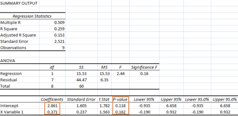
For all regression activities, statistical analysis is a necessity to determine the quality of the fit (how well the regression model fits the data) and the stability of the model (the level of dependence of the model parameters on the particular set of data). The appropriate indicators for such studies are the residual plot (for quality of the fit) and 95% confidence intervals (for stability of the model).
A web-based application for "Multivariate Polynomial Regression (MPR) for Response Surface Analysis" can be found at www.taylorfit-rsa.com. A dataset to test a multivariable regression model is available at UCI Machine Learning Repository contributed by I-Cheng Yeh, "Modeling of strength of high performance concrete using artificial neural networks", Cement and Concrete Research, Vol. 28, No. 12, pp. 1797-1808 (1998). The actual concrete compressive strength [MPa] for a given mixture under a specific age [days] was determined from laboratory. Data is in raw form (not scaled) having 1030 observations with 8 input variables and 1 output variable.
In general, it is difficult to visualize plots beyond three-dimension. However, the relation between output and two variables at a time can be visualized using 3D plot functionality available both in OCTAVE and MATPLOTLIB.
Getting the training data: The evaluation of machine learning algorithm requires set of authentic data where the inputs and labels are correctly specified. However, 'make_blobs' module in scikit-learn is a way to generate (pseudo)random dataset which can be further used to train the ML algorithm. Following piece of code available from jakevdp.github.io/PythonDataScienceHandbook/05.12-gaussian-mixtures.html: Python Data Science Handbook by Jake VanderPlas is a great way to start with.
import matplotlib.pyplot as plt
from sklearn.datasets.samples_generator import make_blobs
X, y = make_blobs(n_samples=400, centers=4, cluster_std=0.60, random_state=0)
X = X[:, ::-1]  # flip axes for better plotting
plt.scatter(X[:, 0], X[:, 1], c=y, s=40, cmap='viridis', zorder=2)
plt.axis('equal')
plt.show()
This generates a dataset as shown below. Note that the spread of data points can be controlled by value of argument cluster_std. 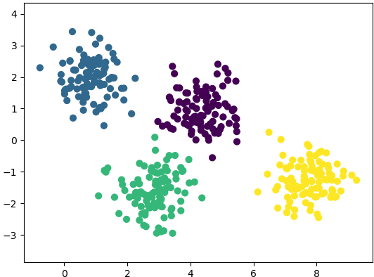
In regression, output variable requires input variable to be continuous in nature. In classifications, output variables require class label and discrete input values.
Under-fitting:
The model is so simple that it cannot represent all the key characteristics of the dataset. In other words, under-fitting is when the model had the opportunity to learn something but it didn't. It is said to have high bias and low variance. The confirmation can come from "high training error" and "high test error" values. In regression, fitting a straight line in otherwise parabolic variation of the data is under-fitting. Thus, adding a higher degree feature is one of the ways to reduce under-fitting. 'Bias' refers to a tendency towards something. e.g. a manager can be deemed biased if he continuously rates same employee high for many years though it may be fair and the employee could have been outperforming his colleagues. Similarly, a learning algorithm may be biased towards a feature and may 'classify' an input dataset to particular 'type' repeatedly. Variance is nothing but spread. As known in statistics, standard deviation is square root of variance. Thus, a high variance refers to the larger scattering of output as compared to mean.Over-fitting:
The model is so detailed that it represents also those characteristics of the dataset which otherwise would have been assumed irrelevant or noise. In terms of human learning, it refers to memorizing answers to questions without understanding them. It is said to have low bias and high variance. The confirmation can come from "very low training error - near perfect behaviour" and "high test error" values. Using the example of curve-fitting (regression), fitting a parabolic curve in otherwise linearly varying data is over-fitting. Thus, reducing the degree feature is one of the ways to reduce over-fitting. Sometime, over-fitting is also described is "too good to be true". That is the model fits so well that in cannot be true.
| ML Performance | If number of features increase | If number of parameters increase | If number of training examples increase |
| Bias | Decreases | Decreases | Remains constant |
| Variance | Increases | Increases | Decreases |
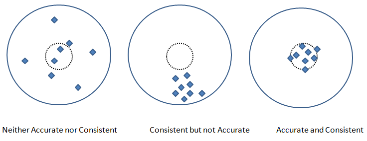
Precision and Recall are two other metric used to check the fidelity of the model. In measurements, 'accuracy' refers to the closeness of a measured value to a standard or known value and 'precision' refers to the closeness of two or more measurements to each other. Precision is sometimes also referred as consistency. Following graphics explains the different between accuracy and precision or consistency.
Pickling
Run the program of learning or training the datasets once and use its parameters every time the code is run again - this process is called pickling (analogous to classical pickles we eat)! In scikit-learn, save the classifier to disk (after training):
from sklearn.externals import joblibjoblib.dump(clf, 'pickledData.pkl')
Load the pickled classifierclf = joblib.load('pickledDatae.pkl')
It is the process of reducing the number of attributes or labels or random variables by obtaining a set of 'unique' or "linearly independent" or "most relevant" or 'principal' variables. For example, if length, width and area are used as 'label' to describe a house, the area can be a redundant variable which equals length × width. The technique involves two steps: [1]Feature identification/selection and [2]Feature extraction. The dimensionality reduction can also be accomplished by finding a smaller set of new variables, each being a combination of the input variables, containing essentially the same information as the input variables. For example, a cylinder under few circumstances can be represented just by a disk where its third dimension, height or length of the cylinder is assumed to be of less important. Similarly, a cube (higher dimensional data) can be represented by a square (lower dimensional data).
- Principal Component Analysis (PCA): This method dates back to Karl Pearson in 1901, is an unsupervised algorithm that creates linear combinations of the original features. The new features are orthogonal, which means that they are linearly independent or uncorrelated. PCA projects the original samples to a low dimensional subspace, which is generated by the eigen-vectors corresponding to the largest eigen-values of the covariance matrix of all training samples. PCA aims at minimizing the mean-squared-error. [Reference: A survey of dimensionality reduction techniques C.O.S. Sorzano, J. Vargas, A. Pascual-Montano] - The key idea is to find a new coordinate system in which the input data can be expressed with many less variables without a significant error.
- Linear Discriminant Analysis (LDA): A "discriminant function analysis" is used to determine which variables discriminate (differentiate or distinguish) between two or more groups or datasets (it is used as either a hypothesis testing or exploratory method). Thus, LDA like PCA, also creates linear combinations of input features. However, LDA maximizes the separability between classes whereas PCA maximizes "explained variance". The analysis requires the data to have appropriate class labels. It is not suitable for non linear dataset.
- Generalized Discriminant Analysis (GDA): The GDA is a method designed for non-linear classification based on a kernel function φ which transform the original space X to a new high-dimensional (linear) feature space. In cases where GDA is used for dimensionality reduction techniques, GDA projects a data matrix from a high-dimensional space into a low-dimensional space by maximizing the ratio of "between-class scatter" to "within-class scatter".
Principal Component Analysis - PCA in OCTAVE
%                                PCA
%PCA: Principal component analysis using OCTAVE -  principal components similar
%to principal stress and strain in Solid Mechanics, represent the directions of
%the data that contains  maximal amount of variance. In  other words, these are
%the lines (in 2D) and planes in (3D) that capture most information of the data.
%Principal components  are less interpretable and may not have any real meaning
%since they are constructed as linear combinations of the initial variables.
%
%Few references:
%https://www.bytefish.de/blog/pca_lda_with_gnu_octave/
%Video on YouTube by Andrew NG
%
 clc; clf; hold off;

% STEP-1: Get the raw data, for demonstration sake random numbers are used

%Generate an artificial data set of n x m = iR x iC size
 iR = 11;  % Total number of rows or data items or training examples
 iC = 2;   % Total number of features or attributes or variables or dimensions
 k  = 2;   % Number of principal components to be retained out of n-dimensions

 X = [2 3; 3 4; 4 5; 5 6; 5 7; 2 1; 3 2; 4 2; 4 3; 6 4; 7 6];
 Y = [  1;   2;   1;   2;   1;   2;   2;   2;   1;   2;   2];
 c1 = X(find(Y == 1), :);
 c2 = X(find(Y == 2), :);
 hold on;
 subplot(211);  plot(X(:, 1), X(:, 2), "ko", "markersize", 8, "linewidth", 2);
 xlim([0 10]); ylim([0 10]);
%
% STEP-2: Mean normalization

% mean(X, 1): MEAN of columns - a row vector {1 x iC}
% mean(X, 2): MEAN of rows - a column vector of size {iR x 1}
% mean(X, n): MEAN of  n-th dimension
  mu = mean(X);

% Mean normalization and/or standardization
  X1 = X - mu;
  Xm = bsxfun(@minus, X, mu);
% Standardization
  SD = std(X);     %SD is a row vector - stores STD. DEV. of each column of [X]
  W = X - mu / SD;

% STEP-3: Linear Algebra - Calculate eigen-vectors and eigen-values
% Method-1: SVD function
% Calculate eigenvectors and eigenvalues of the covariance matrix. Eigenvectors
% are unit vectors and orthogonal, therefore the norm is one and inner (scalar,
% dot) product is zero. Eigen-vectors are direction of principal components and
% eigen-values are value of variance associated with each of these components.

  SIGMA = (1/(iC-1)) * X1 * X1';  % a [iR x iR] matrix
% SIGMA == cov(X')

% Compute singular value decomposition of SIGMA where SIGMA = U*S*V'
  [U, S, V] = svd(SIGMA);   % U is iR x iR matrix, sorted in descending order
% Calculate the data set in the new coordinate system.
  Ur = U(:, 1:k);
  format short G;
  Z = Ur' * X1;
  round(Z .* 1000) ./ 1000;
%
% Method-2: EIG function
% Covariance matrix is a symmetric square matrix having variance values on the
% diagonal and covariance values off the diagonal. If X is n x m then cov(X) is
% m x m matrix. It is actually the sign of the covariance that matters :
% if positive, the two variables increase or decrease together (correlated).
% if negative, One increases when the other decreases (inversely correlated).

% Compute right eigenvectors V and eigen-values [lambda]. Eigenvalues represent
% distribution of the variance among each of the eigenvectors. Eigen-vectors in
% OCTAVE are sorted ascending, so last column is the first principal component.
  [V, lambda] = eig(cov(Xm));  %solve for (cov(Xm) - lambda x [I]) = 0

% Sort eigen-vectors in descending order
  [lambda, i] = sort(diag(lambda), 'descend');
  V = V(:, i);
  D = diag(lambda);

  %P = V' * X;    % P == Z
  round(V .* 1000) ./ 1000;
%
% STEP-4: Calculate data along principal axis
% Calculate the data set in the new coordinate system, project on PC1 = (V:,1)
  x = Xm * V(:,1);
% Reconstruct it and invert mean normalization step
  p = x * V(:,1)';
  p = bsxfun(@plus, p, mu);  % p = p + mu

% STEP-5: Plot new data along principal axis
  %line ([0 1], [5 10], "linestyle", "-", "color", "b");
  %This will plot a straight line between x1, y1 = [0, 5] and x2, y2 = [1, 10]

  %args = {"color", "b", "marker", "s"};
  %line([x1(:), x2(:)], [y1(:), y2(:)], args{:});
  %This will plot two curves on same plot: x1 vs. y1 and x2 vs. y2
  s = 5;
  a1 = mu(1)-s*V(1,1); a2 = mu(1)+s*V(1,1);
  b1 = mu(2)-s*V(2,1); b2 = mu(2)+s*V(2,1);
  L1 = line([a1 a2], [b1 b2]);

  a3 = mu(1)-s*V(1,2); a4 = mu(1)+s*V(1,2);
  b3 = mu(2)-s*V(2,2); b4 = mu(2)+s*V(2,2);
  L2 = line([a3 a4], [b3 b4]);
  args ={'color', [1 0 0], "linestyle", "--", "linewidth", 2};
  set(L1, args{:});  %[1 0 0] = R from [R G B]
  args ={'color', [0 1 0], "linestyle", "-.", "linewidth", 2};
  set(L2, args{:});  %[0 1 0] = G from [R G B]

  subplot(212);
  plot(p(:, 1), p(:, 2), "ko", "markersize", 8, "linewidth", 2);
  xlim([0 10]); ylim([0 10]);
  hold off;
The output from this script is shown below. The two dashed lines show 2 (= dimensions of the data set) principal components and the projection over main principal component (red line) is shown in the second plot.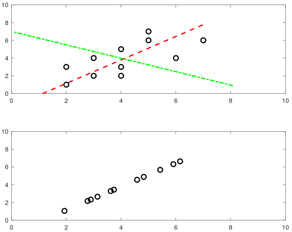
Python install / update
Install / uninstall: do not remove any older version of Python - it may uninstall Ubuntu Desktop as well. In case you unistalled a python which uninstalls Ubuntu desktop, Linux shall start in command line mode only. Use "sudo apt-get update" followed by "sudo apt-get install ubuntu-desktop" to get the desktop re-installed. It should restart with a graphical log-in prompt. If it still opens in command line mode: use 'reboot' command on the prompt. The .bash_profile shall need to be recreated especially for aliases like rm='rm -i', mv='mv -i' and cp='cp -i'.To call Python3 with just 'python' in Linux: sudo rm /usr/bin/python followed by sudo ln -s /usr/bin/python3.9 /usr/bin/python - gives error if link already exists. This way, if Python2.x is needed, it can be called explicitly with python2.x while 'python' defaults to python3 because of the symbolic link. ls -l /usr/bin/python* and ls -l /usr/local/bin/python*- get all installed versions in Linux. To make a specific version default, add in .bash_profile: alias python3='/usr/bin/python3.9'.
Install packages: sudo apt-get install python3-pip, python3 -m pip install matplotlib, pip install numpy, sudo apt-get install python3-opencv. Note that "pip install numpy" works in Linux but prints error message "Access Denied" in Windows. Use "python -m pip install numpy" in Windows terminal.OCTAVE vs. Python
You would have got a flavour of Python programming and OCTAVE script in examples provided earlier. This page does not cover about basic syntax of programming in any of the language. One thing unique in Python is the indentation. Most of the languages use braces or parentheses to define a block of code or loop and does not enforce any indentation style. Python uses indentation to define a block of statements and enforces user to follow any consistent style. For example, a tab or double spaces or triple spaces can be used for indentation but has to be only one method in any piece of code (file).
Following table gives comparison of most basic functionalities of any programming language.
| Usage | OCTAVE | Python |
| Case sensitive | Yes | Yes |
| Current working directory | pwd | import os; os.getcwd() |
| Change working directory | chdir F:\OF | import os; os.chdir("C:\\Users") |
| Clear screen | clc | import os; os.system('cls') |
| Convert number to string | num2str(123) | str(123) |
| End of statement | Semi-colon | Newline character |
| String concatenation | strcat('m = ', num2str(m), ' [kg]') | + operator: 'm = ' + str(m) + ' [kg]' |
| Expression list: tuple | - | x, y, z = 1, 2, 3 |
| Get data type | class(x) | type(x) |
| Floating points | double x | float x |
| Integers | single x | integer x, int(x) |
| User input | prompt("x = ") x = input(prompt) | print("x = ") x = input() |
| Floor of division | floor(x/y) | x // y |
| Power | x^y or x**y | x**Y |
| Remainder (modulo operator) | mod(x,y): remainder(x/y) | x%y: remainder(x/y) |
| Conditional operators | ==, <, >, != (~=), ≥, ≤ | ==, <, >, !=, ≥, ≤ |
| If Loop | if ( x == y ) x = x + 1; endif | if x == y: x = x + 1 |
| For Loop | for i=0:10 x = i * i; ... end | for i in range(1, 10): x = i * i |
| Arrays | x(5) 1-based | x[5] 0-based |
| File Embedding | File in same folder | from pyCodes import function or import pyCodes* as myFile |
| Defining a Function | function f(a, b) ... end | def f(a, b): ... |
| Anonymous (inline) Function | y = @(x) x^2; | y = lambda x : x**2 |
| Return a single random number between 0 ~ 1 | rand(1) | random.random() |
| Return a integer random number between 1 and N | randi(N) | random.randint(1,N) |
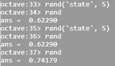
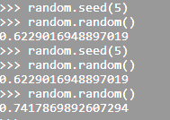
| Return a integer random number with seed | rand('state', 5) | random.seed(5) |
 |  | |
| Return a single random number between a and b | randi([5, 13], 1) | random.random(5, 13) |
| Return a (float) random number between a and b | a + (b-a)*rand(1) | random.uniform(a, b) |
| Return a (float) random number array | rand(1, N) | numpy.random.rand(N) |
| Stop execution after a statement | return | sys.exit() |
To run a function (out of many stored in a module) from the command line: $python3 -c 'import moduleName; funcName()'. The parentheses at the end of funcName makes the function be called. In Windows shell, a double quote should be used instead of single. If funcName() takes arguments, to supply by the command line use sys.argv to the method or access it from the funcName() method. Alternatively, add following lines at the end of module.
if __name__ == "__main__":
  args = sys.argv
  # args[0] = current file (module name), args[1] = function name
  # args[2:] = function args : (*unpacked)
  globals()[args[1]](*args[2:])
Here 'globals' pass the command line argument (name of the function) into locals which is a dictionary with a current local symbol table.
if __name__ == '__main__':
  moduleName()
This is the way to make the function execute (run) when the file is run and not when the file (or module) is imported.
Many use of underscore: throwaway or implicit variable such as "for _ in range(5)", stores the result of the last executed expression (_ allows to call the last function/variable), double leading and trailing underscore such as __variable__ is reserved for special methods, ignoring values such as "_, thresh = cv2.threshold(img, 127, 255, 0)", grouping thousand separator for easy readability of long literals such as 5_000_000.0
Function Annotation: -> marks the (optional) return annotation of a function and annotations are dictionaries. function_name.__annotations__ prints the details such as argument names and type, return values and type...
def func(n: float) -> int:
  return int(n)
print(func.__annotations__) gives output: "{'n': <class 'float'>, 'return': <class 'int'>}". Here the return annotation '->' infers that func() shall return an integer (though the function is not forced to return an integer). The colon separator in "n: float" specifies that 'n' should be of type float. It is like 'int' used while defining a method in (strongly typed language) Java.
public int func(float n) {
  return n * n;
}
Lambda Functions, also known as anonymous functions as they do not have name. They can have any number of arguments but can only have one expression. These are good for one task that needs repetition. Lambda functions can be used inside other regular functions. In fact, this is their main advantage. f = lambda x: x**2 #Like creating a function f, y = f(5) #Execute the function. Some other built-in functions are
zip(a, b) is equivalent to
y = []
for i in range(5):
 for j in range(3):
  if i == j:
   x = (i, j)
   y.append(x)
Ternary Operator
Python for and if on one line: find a list of items matching some criterion - [i for i in xlist if x % 2 == 1]. To find one item matching some criterion, x = next(i for i in xlist if x % 2 == 1). i = next((elm for elm in xlist if elm == 'two'), None) - i will be set to 'None' if there is no matching element. Ternary Operator: result = 'Even' if x % 2 == 0 else 'Odd'.
Tuple and Dictionary
Associative arrays used in other programming languages are called dictionaries in Python. Dictionaries are type of lists where keyrod and value pairs are stored separated by comma. E.g. dictList = {'streams': [{'index': 0, 'codec_name': 'vp9'}, {'index': 1, 'codec_type': 'audio'}], 'format': {'filename': 'in.webm', 'nb_streams': 2}} - this is a list of dictionaries named 'streams' and 'format'. The value of 'codec_type' that is 'audio' can be retrieved by codec = dictList['streams']['codec_name']. In other words, dictionaries are unordered set of key: value pairs, with the requirement that the keys are unique (within one dictionary)
From Python Documentation:- Pair of braces creates an empty dictionary: dictX = {}
- Placing a comma-separated list of key:value pairs within the braces adds initial key:value pairs to the dictionary
- keys() method of a dictionary object returns a list of all the keys used in the dictionary, in arbitrary order
- Apply the sorted() function to it keys() method to get an alphabetically sorted list: sortedKeys = sorted(dictName.keys())
- To check whether a single key is in the dictionary, use the 'in' keyword such as "x not in s" or "y in z"
- To loop through dictionaries, the key and corresponding value can be retrieved at the same time using the iteritems() method: for key, val in dictName.iteritems()
- The dict() constructor builds dictionaries directly from sequences of key-value pairs
- The .get() method retrieves the value associated with a key: keyValue = dictName.get(keyName). If the key exists, it returns the value else Boolean None is returned.
try:
  value = dictName[key]
except KeyError:
  print("Specified key is not present.\n")
  pass
An underscore is used to ignore part of a tuple returned by Python commands: _, dirnames, filenames in os.walk(path) - here the underscore simply tells that the user is not going to use first part of the three-tuple returned by os.walk. However, dpath, dname, fname = os.walk() can be used to access three-tuples returned by os.walk.
Arbitrary Positional Arguments
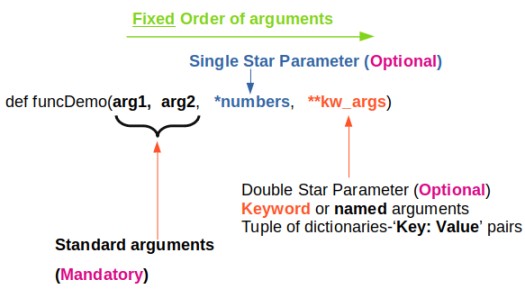
*args and **kwargs allow you to pass arbitrary (multiple) positional arguments and arbitrary (multiple) keyword arguments respectively to a function without declaring them beforehand. Note that keyword arguments are like dictionary with a 'key=value' pair where = is used instead of colon (:). The star (*) and double-stars (**) respectively at the start of these names are called asterisk operators or unpacking operators which return iterable objects as tuple. A tuple is similar to a list in that they both support slicing and iteration. Note that tuples are not mutable that is they cannot be changed. Tuples are specified as comma separated items inside parentheses like theTuple = (1, 2, 3) whereas lists are specified in brackets like theList = [1, 2, 3].
args[0] or "for arg in args" and kwargs[kwrd] or "for key, value in kwargs.items()" or "for kwval in kwargs.values()" can be used to access each members of args and kwargs lists respectively. "for key in kwargs" can be used to access 'key' names in kwargs list comprising of pairs of keywords and values.
How to check if *args[0] exists? Note that *args is a tuple (with zero, one or more elements) and it will result in a True if it contains at least one element. Thus, the presence of *args can be simply checked by "if args:" Similarly, if 'key1' in kwargs: can be used if key1 in **kwargs exists or not? len(args) ≡ args.__len__() and len(kwargs): find length of positional arguments. How to check if function is callable with given *args and **kwargs? While looping through a sequence, the position index and corresponding value can be retrieved at the same time using the enumerate() function: for idx, val in enumerate(listName)
Arrays
aRaY = [] - here aRaY refers to an empty list though this is an assignment, not a declaration. Python can refer aRaY to anything other than a list since Python is dynamically typed. The default built-in Python type is called a 'list' and not an array. It is an ordered container of arbitrary length that can hold a heterogeneous collection of objects (i.e. types do not matter). This should not be confused with the array module which offers a type closer to the C array type. However, the contents must be homogenous (all of the same type), but the length is still dynamic.This file contains some examples of array operations in NumPy.
arr = np.array( [ [0, 0, 0, 0], [0, 1, 1, 0], [0, 1, 1, 0], [0, 0, 0, 0] ] )print(arr): output is
[[0 0 0 0]
 [0 1 1 0]
 [0 1 1 0]
 [0 0 0 0]]
print(type(arr)) = <class 'numpy.ndarray'>
x = np.array([1.2, 2.3, 5.6]), x.astype(int) = array([1, 2, 6])
row_vector = array([[1, 3, 5]]) or np.r_['r', [1, 3, 5]] which has 1 row and 3 columns, col_vector = array([[2, 4, 6]]).T or np.r_['c', [2, 4, 6]] which has 3 rows and 1 column. Convert a row vector to column vector: col_vec = row_vec.reshape(row_vec.size, 1), or col_vec = row_vec.reshape(-1, 1) where -1 automatically finds the value of row_vec.size. Convert a column vector to row vector: row_vec = col_vec(1, -1). Examples:a = np.linspace(1, 5, num=5) > print(a) >> [1. 2. 3. 4. 5.] print(a.shape) >> (5,) print(a.reshape(-1, 1)) [[1.] [2.] [3.] [4.] [5.]] print((a.reshape(-1, 1)).shape) >> (5, 1) x = np.array([1,2,3,4,5]) > print(x) >> [1 2 3 4 5]. print(x.shape) >> (5,) x = np.array([[1,2,3,4,5]]) > print(x.shape) >> (1, 5) x = np.arange(1, 5, 1) > print(x) >> [1 2 3 4]. print(x.shape) >> (4,)2D operations
X = np.array([1, 2, 3]), Y = np.array([2, 4, 6]), X, Y = np.meshgrid(X, Y)
Z = (X**2 + Y**2), print(Z)
[[ 5  8 13]
 [17 20 25]
 [37 40 45]]
i.e. Z = np.array([[5, 8, 13], [17, 20, 25], [37, 40, 45]])
Summary
Python interpreter is written in C language and that array library includes array of C language. A string is array of chars in C and hence an array cannot be used to store strings such as file names.
- Floating-point arithmetic always produces a floating-point result. Hence, modulo operator for integers and floating point numbers will yield different results.
- Python uses indentation to show block structure. Indent one level to show the beginning of a block. Outdent one level to show the end of a block. The convention is to use four spaces (and not the tab character even if it is set to 4 spaces) for each level of indentation. As an example, the following C-style code:
C                       Python
if (x > 0) {            if x:
 if (y > 0)  {              if y:
        z = x+y                 z = x+y
    }                       z = x*y
    z = x*y
}
Comments: Everything after "#" on a line is ignored. Block comments starts and ends with ''' in Python. - eye(N), ones(N) and zeros(N) creates a NxN identity matrix, NxN matrix having each element '1' and NxN matrix having each element '0' respectively.
- 'seed' number in random number generators is only a mean to generate same random number again and again. This is equivalent to rng(5) in MATLAB.
- linspace(start, end, num): num = number of points. If omitted, num = 100 in MATLAB/OCTAVE and num = 50 in numpy. Note that it is number of points which is equal to (1 + number of divisions). Hence, if you want 20 divisions, set num = 21. That is, increment Δ = (end - start) / (num - 1). Available in numpy, OCTAVE/MATLAB.
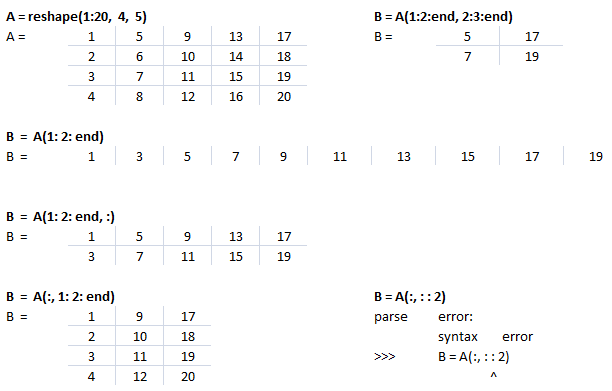
- linspace(1, 20, 20) = 1:20. And hence, reshape(1:20, 4, 5) is equivalent to reshape(linspace(1, 20, 20), 4, 5)
- Arrays: use space or commas to delimit columns, use semi-colon to delimit rows. In same ways, space can be used to stack arrays column-wise (hstack in numpy) e.g. C = [A B] and semi-colon can be used to stack arrays row-wise (vstack in numpy) e.g. C = [A; B].
- In numpy, if x is a 2D array then x[0,2] = x[0][2]. NumPy arrays can be indexed with other arrays. x[np.array([3, 5, 8])] refers to the third, fifth and eighth elements of array x. Negative values can also be used which work as they do with single indices or slices. x[np.array([-3, -5, -8])] refers to third, fifth and eighth elements from the end of the vector 'x'.
- Negative indexing to call element of an array or a matrix is not allowed in OCTAVE/MATLAB. In case negative counters of a loop is present e.g. j = -n:n, use i = 1:numel(j) to access x(i).
Conditional and Logical Indexing
u(A < 25) = 255 replaces the elements of matrix 'u' to 255 corresponding to elements of A which is < 25. If A = reshape(1:20, 4, 5) then B = A(A>15)' will yield B = [16 17 18 19 20]. B = A; B(A < 10) = 0 will replace all those elements of matrix A which are smaller than 10 with zeros.B = A < 9 will produce a matrix B with 0 and 1 where 1 corresponds to the elements in A which meets the criteria A(i, j) < 9. Similarly C = A < 5 | A > 15 combines two logical conditions.
Find all the rows where the elements in a column 3 is greater than 10. E.g. A = reshape(1:20, 4, 5). B = A(:, 3) > 10 finds out all the rows when values in column 3 is greater than 10. C = A(B:, :) results in the desired sub-matrix of the bigger matrix A.vectorization
This refers to operation on a set of data (array) without any loop. Excerpts from OCTAVE user manual: "Vectorization is a programming technique that uses vector operations instead of element-by-element loop-based operations. To a very good first approximation, the goal in vectorization is to write code that avoids loops and uses whole-array operations". This implicit element-by-element behaviour of operations is known as broadcasting.Summation of two matrices: C = A + B
for i = 1:n
  for j = 1:m
    c(i,j) = a(i,j) + b(i,j);
  endfor
endfor
Similarly:
for i = 1:n-1
  a(i) = b(i+1) - b(i);
endfor
can be simplified as a = b(2:n) - b(1:n-1)
If x = [a b c d], x .^2 = [a2 b2 c2 d2]
The vector method to avoid the two FOR loops in above approach is: C = A + B where the program (numPy or OCTAVE) delegates this operation to an underlying implementation to loop over all the elements of the matrices appropriately.
Slicing
This refers to the method to reference or extract selected elements of a matrix or vector. Indices may be scalars, vectors, ranges, or the special operator ':', which may be used to select entire rows or columns. ':' is known as slicing object. The basic slicing syntax is "start: stop: step" where step = increment. Note that the 'stop' value is exclusive that is rows or columns will be included only up to ('stop' - 1). In NumPy (and not in OCTAVE), any of the three arguments (start, stop, step) can be omitted. Default value of 'step' = 1 and default value of 'start' is first row or column. In NumPy (not in OCTAVE) an ellipsis '...' can be used to represent one or more ':'. In other words, an Ellipsis object expands to zero or more full slice objects (':') so that the total number of dimensions in the slicing tuple matches the number of dimensions in the array. Thus, for A[8, 13, 21, 34], the slicing tuple A[3 :, ..., 8] is equivalent to A[3 :, :, :, 8] while the slicing tuple A[..., 13] is equivalent to A[:, :, :, 13]. Special slicing operation A[::-1] reverses the array A. Note that even though it is equivalent to A[len(A)-1: -1: -1], the later would produce an empty array.
Slicing to crop an image: img_cropped = img(h0: h0+dh, w0: w0+dw) can be used to crop an image (which is stored as an array in NumPy). This one line code crops an array by number of pixels w0, h0, dw and dh from left, top, right and bottom respectively. Similarly, the part of an array (and hence an image) can be replaced with another image in this one line of code: img_source(h0: h0 + img_ref.shape[0], w0: w0 + img_ref.shape[1]) = img_ref -> here the content of image named img_ref is replaced inside img_source with top-left corner placed at w0 and h0 in width and height directions respectively.Slicing against column: B = A(3:2:end, :) will will slice rows starting third row and considering every other row thereafter until the end of the rows is reached. In numpy, B = A[:, : : 2] will slice columns starting from first column and selecting every other column thereafter. Note that the option ': : 2' as slicing index is not available in OCTAVE.
Let's create a dummy matrix A = reshape(1:20, 4, 5) and do some slicing such as B = A(:, 1:2:end). 
This text file contains example of Slicing in NumPy. The output for each statement has also been added for users to understand the effect of syntaxes used. There is a function defined to generate a sub-matrix of a 2D array where the remaining rows and columns are filled with 255. This can be used to crop a portion of image and filling the remaining pixels with white value, thus keeping the size of cropped image of size as the input image.
Arrays: Example syntax and comparison between OCTAVE and NumPy
| Usage | GNU OCTAVE | Python / NumPy |
| Definition | A = reshape(0:19, 4, 5)' | A = numpy.arange(20).reshape(5, 4) |
| Reshape example | 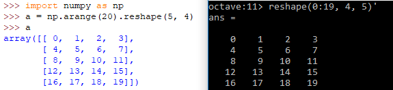 | |
| A(3) | Scalar - single element | - |
| A[3] | Not defined | Same as A[3, :]: 4th row of matrix/array |
| Special arrays | zeros(5, 8), ones(3,5,"int16") | np.zeros( (5, 8) ), np.ones( (3, 5), dtype = np.int16) |
| Create array from txt files | data = dlmread (fileName, ".", startRow, startCol) | np.genfromtxt(fileName, delimiter=",") |
3D arrays: widely used in operations on images
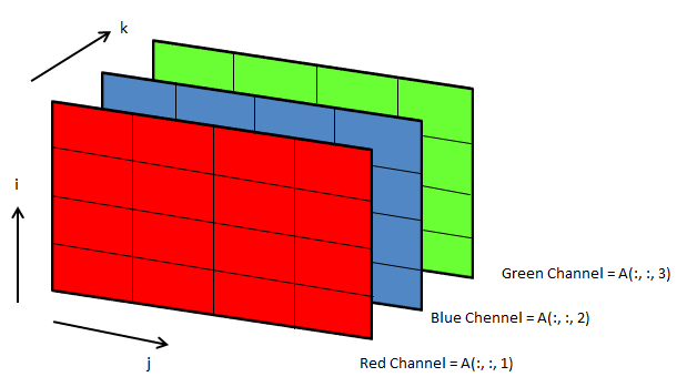
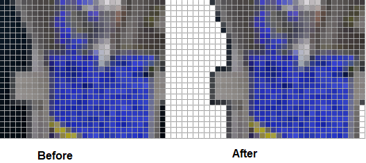
Following OCTAVE script can be used to convert the background colour of an image from black to white.
clc; clear; clear all; [x, map, alpha] = imread ("Img.png"); [nR nC nZ] = size(x);

A = x(:, :, 1); B = x(:, :, 2); C = x(:, :, 3); i = 40; u = A; v = B; w = C;
u(A<i & B<i & C<i) = 255; v(A<i & B<i & C<i) = 255; w(A<i & B<i & C<i) = 255;

z = cat(3, u, v, w); imwrite(z, "newImg.png"); imshow(z);
File Operations in Python
- List files and folders: dirpath, subdirs, files = os.walk(root_folder) - os.walk returns a three-tuple (dirpath, dirnames, filenames) where dirpath is nothing but the top-level root folder specified, subdirs = sub-directories below root folder. Thus, "for dirpath, subdirs, files in os.walk(root_folder)" will create one outer loop (list or names of sub-folders) and an inner loop (list or names of files in each sub-folder).
- As per user doc: "Note that the names in the lists contain no path components. To get a full path (which begins with top) to a file or directory in dirpath, do os.path.join(dir_path, file_name). Whether or not the lists are sorted depends on the file system."
- Sort a list: files.sort(), to list them in numeric order: sorted(files, key=int). os.walk() yields in each step what it will do in the next step(s).
- Find number of folders: n_dirs = sum([ len(dirs) for root, dirs, files in os.walk(root_folder) ])
- Number of files: n_files = sum([ len(files) for root, dirs, files in os.walk(root_folder) ])
- Check if a file exists: os.path.isfile(fileName)
- Check if a folder exists: os.path.isdir(str(dirPath))
- Get file extension: f_extn = fileName.partition('.')[-1]
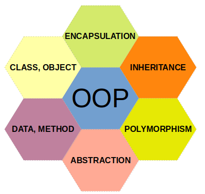
Procedural or Functional Programming vs. Object Oriented Programming - Functional programs tend to be a bit easier to follow than OOP which has intricate class hierarchies, dependencies and interactions. From learn.microsoft.com titled getting-started-with-vba-in-office: "Developers organize programming objects in a hierarchy, and that hierarchy is called the object model of the application. The definition of an object is called a class, so you might see these two terms used interchangeably. Technically, a class is the description or template that is used to create, or instantiate, an object. Once an object exists, you can manipulate it by setting its properties and calling its methods. If you think of the object as a noun, the properties are the adjectives that describe the noun and the methods are the verbs that animate the noun. Changing a property changes some quality of appearance or behavior of the object. Calling one of the object methods causes the object to perform some action."
A related concept is namespace which is a way of encapsulating items. Folders are namespace for files and other folders.
As a convention, an underscore _ at the beginning of a variable name denotes private variable in Python. Note that it is a convention as the concept of "private variables" does not exist in Python.
Class definition like function 'def' statement must be executed before used.#!/usr/bin/env python3
import math
class doMaths(): # definition of a new class
py = 3.1456 # can be accessed as doMaths.py
# Pass on arguments to a class at the time of its creation using
# __init__ function.
def __init__(self, a, b):
# Here 'self' is used to access the current instance of class, need
# not be named 'self' but has to be the first parameter of function
# Define a unique name to the arguments passed to __init__()
self.firstNum = a
self.secondNum = b
self.sqr = a*a + b* b
self.srt = math.sqrt(a*a + b*b)
print(self.sqr)
def evnNum(self, n):
if n % 2 == 0:
print(n, " is an even number \n")
else:
print(n, " is an odd number \n")
# Create an INSTANCE of the class doMaths: called Instantiate an object
xMath = doMaths(5, 8) # Output = 89
print(xMath.firstNum) # Output = 5
print(xMath.sqr) # Output = 89
# Access the method defined in the class
xMath.evnNum(8) # Output = "8 is an even number"
class doMaths(mathTricks) - here 'doMaths' class is inherited from class 'mathTricks'. When a __init__() function is added in the child class it will no long inherit the parent's __init__() function. This is called overriding the inheritance. To keep the inheritance, call parent's __init__(0 as parentClassName.__init__() such as mathTricks.__init__() in this case. Alternatively, one can use super() function. While child class (doMaths here) inherits all attributes and method definitions of parent class (mathTricks here), new attributes and methods specific to child class can be added as per the requirements. However, method with the same name and arguments in chile or derived class and parent or base or super class, the method in derived class overrides the method in the base class: this is known as Method Overriding.
Decorators: There are functions that take a function and returns some value by adding new functionalities. A decorator is assigned by adding @ before the name. Adding a decorator before a function, Python calls the function without assigning the function call to a variable. e.g.
@decore_func
def next_func():
  ...
If y = next_func() is called, next_func() ≡ y = decor_func(next_func). Multiple decorators can be chained by placing one after the other, most inner being applied first. Special decorator @property is used to define 'property' of a 'class' object. For example:
class personalData:
  ...
  @property
  def personName(self):
    return self.name
  ...
  ...
It sets personName() function as a property of a class personalData.
Python Argument Parsing
Python functions are a great way to make your code modular and granular. One can store many functions in a Python code file and pass arguments through command line using argparse module. The sample code below demonstrates how multiple functions can be called based on desired operation and arguments can be passed to each of the functions called. Either sys.argv or argparse can be used to achieve same objectives though arparse tend to be more convenient. As argparse automatically checks the presence of arguments, the conditional statements needed in sys.argv is not required with argparse. Argparse can automatically generate usage and help messages.
Excerpt from stackoverflow.com/ ~ /use-argparse-to-run-1-of-2-functions-in-my-script: If a python file is intended to be accessed in multiple ways (called as a script, loaded as a module from another python file), then the parts specific to "being run as a script" should be in your main-section. You can write a function main() and call that in a __name__ == "__main__" if block, or write your script action code directly in said if block.
Argument Parsing is a necessary step to create Command Line Interface (CLI). One can create sub-commands, add options or flags or switches using argument parsing. In example "pip install -r list.txt", install is a sub-command to main command pip, -r is an option to subcommand 'install' and list.txt is parameter to option. Note that argparse parses all arguments at once and no conditional parsing based on arguments is feasible. Alternatively, "Python Fire" is a library for automatically generating command line interfaces (CLIs) from absolutely any Python object. Fire can call a function without changing the script: python -m fire moduelName funcName. It also has a built-in argparser.
import argparse
if __name__ == "__main__":
  parser = argparse.ArgumentParser(prog='pyArgParsing',
                    description='Edit PDF Files using PyPDF2',
                    epilog='Delete, rotate and scale pages of a PDF')

  # Attach individual argument specifications to the parser: add_argument
  parser.add_argument("operation", help="Operation to be performed", \
                      choices=["delete","shuffle","scale"])
  parser.add_argument("file_name", help="Input PDF File Name")
  parser.add_argument("startPage", help="Start page number")
  parser.add_argument("endPage", help="End page number")

  # Optional arguments: '*' or '+'- All command-line arguments are gathered
  # into a list. nargs='argparse.REMAINDER': All the remaining command-line
  # arguments are gathered into a list. args='?' - does not produce a list.
  # nargs=N, N arguments from the command line collected into a list
  parser.add_argument('scale', nargs='?', default=1.0)

  args = parser.parse_args()

  if args.operation == "delete":
    deletePagesPDF(args.file_name, int(args.startPage), int(args.endPage))
  elif args.operation == "shuffle":
    shufflePagesPDF(args.file_name, int(args.startPage), int(args.endPage))
  elif args.operation == "scale":
    s=float(args.scale)
    scalePagesPDF(args.file_name, int(args.startPage), int(args.endPage), s)
Note that nargs creates a list except nargs='?'. Hence, if a function takes string as argument, such as path of a folder, do not use nargs. Else, you may get error "TypeError: stat: path should be string, bytes, os.PathLike or integer, not list". This code can be run from command line as: python3 pyArgParsing.py delete input.pdf 3 8 and python3 pyArgParsing.py scale input.pdf 3 8 1.5
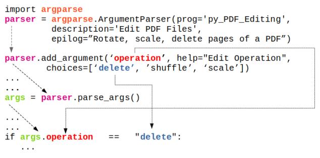
From docs.python.org/3/library/argparse.html
import argparse

parser = argparse.ArgumentParser(description='Process some integers.')
parser.add_argument('integers', metavar='N', type=int, nargs='+',
                    help='an integer for the accumulator')
parser.add_argument('--sum', dest='accumulate', action='store_const',
                    const=sum, default=max,
                    help='sum the integers (default: find the max)')

args = parser.parse_args()
print(args.accumulate(args.integers))

$- python3 testArgParser.py
usage: testArgParser.py [-h] [--sum] N [N ...]
testArgParser.py: error: the following arguments are required: N

$- python3 testArgParser.py -h
usage: testArgParser.py [-h] [--sum] N [N ...]

Process some integers.

positional arguments:
  N           an integer for the accumulator

optional arguments:
  -h, --help  show this help message and exit
  --sum       sum the integers (default: find the max)

$- python3 testArgParser.py 1 2 3 4
4

$- python3 testArgParser.py 1 2 3 4 --sum
10
Reference: docs.python.org/3/library/argparse.html
prefix_chars: Most command-line options will use hyphen - as the prefix, e.g. -name or --name. Parsers that need to support different or additional prefix characters, e.g. for options like +name or /name, may specify them using the prefix_chars= argument to the ArgumentParser constructor: parser = argparse.ArgumentParser(prog = 'denoiseImages', prefix_chars='-+'). The prefix_chars= argument defaults to '-'. Supplying a set of characters that does not include '-' will cause -name or --name options to be disallowed.There are two types of arguments: [1] positionals: these are identified by order without any identifying name and [2] optionals: these are identified by a name or flag string such as parser.add_argument("-name") or parser.add_argument("--name"). The order of optionals does not matter and optionals are similar (but not identical) to the keyword arguments of Python functions. By default, ArgumentParser groups command line arguments into "positional arguments" and 'options' displaying messages. Argument groups can be used in case such default grouping does not help.
parser.add_argument("-name"): the command line arguments should be entered as "-name Krishna". parser.add_argument("--name"): the command line arguments should be entered as "--name Krishna". In case multiple entries are made such as "-name Ram -name Krishna", the last entry shall be used by the argument parser.
parser.add_argument("-x", "--del", action="store_true"): option names start with - for shorthand flags and -- for long flags. Action argument "store_true" accompanies option indicate that this option will be stored as Boolean value. If the option at the command line is provided, its value will be True else False.
Arguments shared between parsers: There are many instances where arguments are shared across different parsers. To avoid repeating the definitions of such shared arguments, "parent=" argument to ArgumentParser can be used.
![]()
Sub-commands
Reference: docs.python.org/3.2/library/argparse.html --- Many programs split up their functionality into a number of sub-commands, a particularly good idea when a program performs several different functions which require different kinds of command-line arguments. ArgumentParser supports the creation of such sub-commands with the add_subparsers() method. The add_subparsers() method is normally called with no arguments and returns a special action object.
import argparse, sys
# Adaptation of example at docs.python.org/3/library/argparse.html#sub-commands

# Sub-command functions
def sub_cmd1(args) :
  print(args.x * args.y)

def sub_cmd2(args):
  print(args.u + args.v)

# Create the top-level parser
parser = argparse.ArgumentParser()
subparsers = parser.add_subparsers(required=True)

# Create the (sub) parser for the 'sub_cmd1' command
parser_sub_cmd1 = subparsers.add_parser('sub_cmd1')
parser_sub_cmd1.add_argument('-x', type=int, default=10)
parser_sub_cmd1.add_argument('y', type=float )
parser_sub_cmd1.set_defaults(func = sub_cmd1)

# Create the (sub) parser for the 'sub_cmd2' command
parser_sub_cmd2 = subparsers.add_parser('sub_cmd2')
parser_sub_cmd2.add_argument('-u', type=int, default=10)
parser_sub_cmd2.add_argument('v', type=int)
parser_sub_cmd2.set_defaults(func = sub_cmd2)

# Parse the arguments and call whatever function was specified on command line
if len(sys.argv) > 1:
  args = parser.parse_args()
  args.func(args)
else:
  print("\n  ---No sub-command name provided. \n")
Usage:
python3 cmd_sub.py sub_cmd1
  usage: cmd_sub.py sub_cmdi [-h] [-x X] y
  cmd sub.py sub cmd1: error: the following arguments are required: y
python3 cmd_sub.py sub_cmd1 3: output = 30.0, python3 cmd _sub.py sub_cmd1 -x 10 25: output = 250.0, python3 cmd_sub.py sub_cmd2 5: output = 15, Python3 cmd_sub.py sub_cmd2 -u 4 5: output = 9
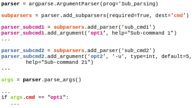
Note that the sub-commands used in above example are the names of the 'functions'. If sub-commands are intended to be a 'switch' to activate a particular loop or conditional statement of a function, following example can be used. Here, 'files' and 'folder' are mere options to be passed on to the function mergePDF().
parser = argparse.ArgumentParser()
subparsers = parser.add_subparsers(dest="command")

# Create the (sub) parser for the 'files' command
parser_files = subparsers.add_parser('files',
                                 help="Merge files specified on command line")
parser_files.add_argument('-f', nargs='*')

# Create the (sub) parser for the 'folder' command
parser_folder = subparsers.add_parser('folder',
                                 help="Merge PDF files in specified directory")
parser_folder.add_argument('-d', nargs=1)

# Parse the arguments and call whatever function was specified on command line
args = parser.parse_args()
if args.command == 'files':
  if args.f:
    mergePDF(0, args.f)
elif args.command == 'folder':
  if args.d:
      mergePDF(1, args.d[0])
else:
  print("\n  ---No sub-command name provided. \n")
The complete code can be found in this file.
Sub-sub-command: sometimes we need to have a main command followed by additional multiple sub-commands as described below.
mainScript.py  Command    Sub-commands       Arguments
-------------  ---------  -----------------  ----------------------------------
               mergePDF
                          mergeFiles         f1, f2, ...
                          mergeInFolder      folderName
               editPDF
                          deletePages        f, sPg, nPg...
                          rotatePages        f, sPg, nPg, q...
                          scalePages         f, sPg, nPg, s...
                          cropPages          f, sPg, nPg, wL, wT, wR, wB...
The generic implementation can be found in this file.
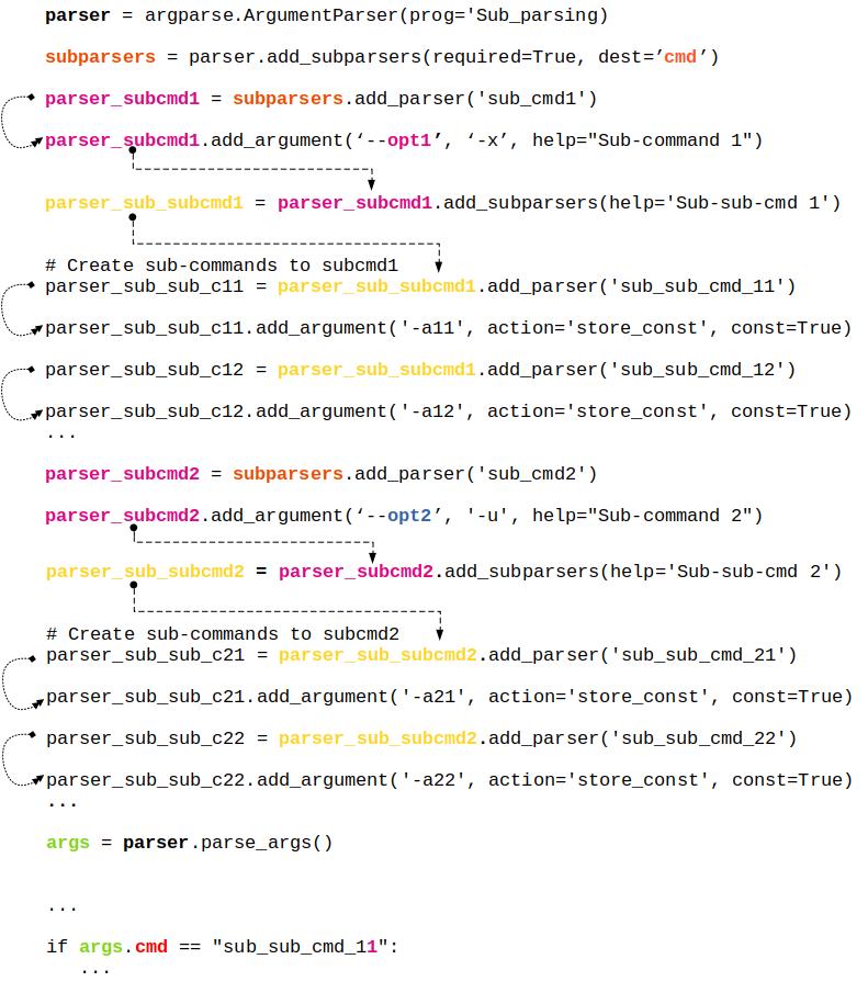
Summary of 'action' keyword
| Action Keyword | Action Performed by Argparser | Remark |
| store | This just stores the argument’s value | This is the default action |
| store_const | This stores the value specified by the const keyword which defaults to None. | Commonly used with optional arguments to specify some sort of flag |
| store_true | Special case of 'store_const' | To store the value True |
| store_false | Special case of 'store_const' | To store the value False |
| append | Stores a list, and appends each argument value to the list | It is useful to allow an option to be specified multiple times |
| append_const | Stores a list, and appends the value specified by the const keyword argument to the list | Useful when multiple arguments need to store constants to the same list |
| count | Counts the number of times a keyword argument occurs | For example, this is useful for increasing verbosity levels |
| help | Prints a complete help message for all the options in the current parser and then exits. | By default a help action is automatically added to the parser |
| version | Prints version information and exits when invoked | This expects a 'version=' keyword argument in the add_argument() call |
| extend | Stores a list, and extends each argument value to the list | Similar to 'append' |
The information tabulated above is just a re-formatting of text available at docs.python.org/3/library/argparse.html
Few Tips: re-organized from official documentation
- ArgumentParser, by default groups arguments into positional arguments and options when displaying help messages. add_argument_group() method can be used to group arguments as per user-defined category which displays arguments in separate groups in help messages.
- When parsers share a common set of arguments, the definitions of these arguments does not need to be repeated by using a single parser with all the shared arguments and passed to parents= argument to ArgumentParser. Such parent parsers must specify add_help=False to prevent conflicting help messages.
- To globally suppress attribute creation on parse_args() calls, parser = argparse.ArgumentParser( argument_default = argparse.SUPPRESS ).
- By default, for positional argument actions, the dest value is used directly, and for optional argument actions, the dest value is uppercased.
- metavar can be used to change the displayed name of an argument and a tuple can be provided to metavar to specify different display names for each of the arguments.
- As evident, hyphen '-' is used for positional arguments or can be used to specify a negative value to an argument. parse_args() method takes the convention: "positional arguments may only begin with - if they look like negative numbers and there are no options in the parser that look like negative numbers".
Linear algebra deals with system of linear algebraic equations where the coefficients of independent variables {x} are stored as a matrix [A] and the constant terms on the right hand side of equations are stored as a column vector {b}.
| Usage | OTAVE | Python (NumPy) |
| Array Index | 1-indexed | 0-indexed |
| Inverse of a square matrices (a 2D array in numPy) | inv(A) | inv(A) |
| Find the solution to the linear equation [A].{x} = {b} | x = linsolve (A, b) or x = A \ b or x = mldivide (A, b) | solve(A, b) |
| Eigen-values (V) and eigen vectors (λ): [A].{x} = λ{x} | [V, lambda] = eig (A) | eigvals(A): only eigen-values, eig(A): both eigen-values & eigen-vectors |
| Determinant of an array: product of singular values of the array | det(A) | det(A) |
| Generalized pseudo-inverse of A which is same as the inverse for invertible matrices | pinv(A, tol) | pinv(A) |
| The rank of a matrix is the number of linearly independent rows or columns and determines how many particular solutions exist to a system of equations. OCTAVE compute the rank of matrix A using the singular value decomposition. | ||
| Rank: number of singular values of A > specified tolerance tol | rank(A, tol) | (x, resids, rank, s) = lstsq (A, b, tol) |
| Cholesky decomposition, L of A such that A = LLH | chol(A, "lower") | cholesky (A): by default it computes lower triangular matrix |
Statistics
This topics includes basic descriptive statistics, probability distribution functions, hypothesis tests, design-of-experiments (DOE), random number generation ... Descriptive statistics refers to the methods to represent the essence of a large data set concisely such as the mean (average of all the values), median (the value dividing the dataset in two halves), mode (most frequently occurring value in a dataset), range (the difference between the maximum and the minimum of the input data)... functions which all summarize a data set with just a single number corresponding to the central tendency of the data.
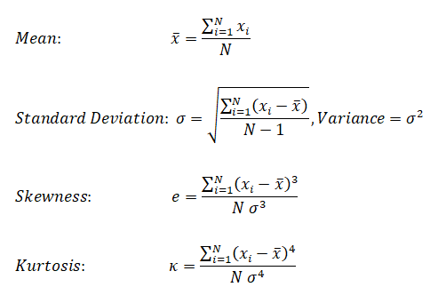
Median is the 50 percentile, the value that falls in the middle when the observations are sorted in ascending of descending order. While standard deviation is a measure of central tendency, skewness is the measure of assymetry (skew or bias in the data). Kurtosis is measure of deviation from normal distribution.
| Evaluation parameter | OTAVE | Python (numPy) |
| Mean (average) | mean(x) | mean(x) |
| Median (value that divides dataset) | median(x) | median(x) |
| Mode (most frequently occurring value) | mode(x) | mode(x) |
| Range | range(x) | ptp(x) |
| Mean of squares | meansq(x) | - |
| Variance | var(x) | var(x) |
| Standard deviation | std(x) | std(x) |
| Skewness | skewness(x) | skew(x)* |
| Kurtosis | kurtosis(x) | kurtosis(x)* |
| All-in-one | statistics (x) | describe(x) |
statistics(x): OCTAVE returns a vector with the minimum, first quartile, median, third quartile, maximum, mean, standard deviation, skewness, and kurtosis of the elements of the vector x.
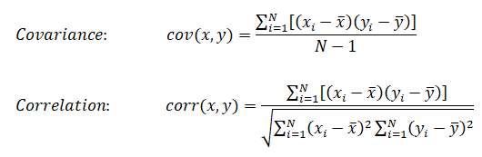
Cheat-sheet: R-programming
- Get help on any specific named function, for example solve, use: help(solve). An alternative is: > ?solve
- R is an expression language and is case sensitive
- Commands are separated either by a semi-colon (‘;'), or by a newline. Elementary commands can be grouped together into one compound expression by braces ‘{' and ‘}'.
- Comments can be put almost anywhere, starting with a hashmark (‘#'), everything to the end of the line is a comment.
- If a command is not complete at the end of a line, R will give a different prompt, by default '+' on second and subsequent lines and continue to read input until the command is syntactically complete.
- If commands are stored in an external file, say commands.r in present working directory: source("commands.r")
- The function sink("record.list") will divert all subsequent output from the console to an external file, record.lis
- The command sink() restores it to the console once again
- Variable assignment is by either of 3 operators: equal operator '=', leftward operator "<-", rightward operator "->"
- Arrays: c() function which means to combine the elements into a vector. fruits <- c("banana", "apple", "mango"). In R - matrix is a two-dimensional rectangular data set, arrays can be of any number of dimensions set by dim attribute.
- Colon operator - Similar to OCTAVE, ':' creates a series of numbers in sequence for a vector. e.g. v <- 1:5 will create v = (1 2 3 4 5)
- Loops: the syntax for Loops in R is similar to that in C.
- Plots: the plot command in R is similar to that in OCTAVE or MATLAB - plot(x, y). Method to add color and title are different than OCTAVE: color = "green", main = "Chart Tile" is used to specify color of plot and title of the plot respectively.
- In OCTAVE, subplot(231) creates an array of 2x3 = 6 plots. The third digit specifies location of image in 2x3 matrix. In R, mfcol = c(3, 2) sets multiple figure environment and mfg = c(3, 2, 1, 1) specified position of the current figure in a multiple figure environment.
- Reading database
Following plots are generated in GNU OCTAVE script described later.
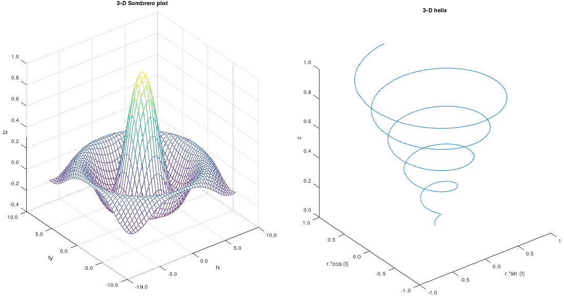
%Examples of 3D plots
%-------------------- -------------------------- ------------------------------
%  3D Somerero Plot
figure ();

subplot (1,2,1);
tx = ty = linspace(-8, 8, 41)';
[xx, yy] = meshgrid(tx, ty);
r = sqrt(xx .^ 2 + yy .^ 2) + eps;
tz = sin(r) ./ r;

mesh(tx, ty, tz);
xlabel("tx"); ylabel("ty"); zlabel("tz");
title("3-D Sombrero plot");

% Format X-, Y- and Z-axis ticks
xtick = get(gca,"xtick"); ytick = get(gca,"ytick");  ztick = get(gca,"ztick");
xticklabel = strsplit (sprintf ("%.1f\n", xtick), "\n", true);
set (gca, "xticklabel", xticklabel)
yticklabel = strsplit (sprintf ("%.1f\n", ytick), "\n", true);
set (gca, "yticklabel", yticklabel);
zticklabel = strsplit (sprintf ("%.1f\n", ztick), "\n", true);
set (gca, "zticklabel", zticklabel);
%-------------------- -------------------------- ------------------------------
%  3D Helix
subplot(1,2,2);
t = 0:0.1:10*pi;
r = linspace(0, 1, numel(t));  % numel(t) = number of elements in object 't'
z = linspace(0, 1, numel(t));
plot3(r.*sin(t), r.*cos(t), z);
xlabel("r.*sin (t)"); ylabel("r.*cos (t)"); zlabel("z");
title("3-D helix");

% Format X-, Y- and Z-axis ticks
xtick = get(gca,"xtick"); ytick = get(gca,"ytick");  ztick = get(gca,"ztick");
xticklabel = strsplit (sprintf ("%.1f\n", xtick), "\n", true);
set (gca, "xticklabel", xticklabel)
yticklabel = strsplit (sprintf ("%.1f\n", ytick), "\n", true);
set (gca, "yticklabel", yticklabel);
zticklabel = strsplit (sprintf ("%.1f\n", ztick), "\n", true);
The Python code to generate the 3D Helix is as follows.
import matplotlib as mpl; import matplotlib.pyplot as plt
from mpl_toolkits.mplot3d import Axes3D; import numpy as np
#-------------------- -------------------------- ------------------------------
mpl.rcParams['legend.fontsize'] = 10

fig = plt.figure(); ax = fig.gca(projection='3d')
t = np.linspace(0, 10 * np.pi, 100); r = np.linspace(0, 1, np.size(t));
z = np.linspace(0, 1, np.size(t));   x = r * np.sin(t); y = r * np.cos(t)

ax.plot(x, y, z, label='3D Helix');  ax.legend(); plt.show()
The Python code to generate the 3D Somerero Plot is as follows.
from mpl_toolkits.mplot3d import Axes3D; import numpy as np
import matplotlib.pyplot as plt; from matplotlib import cm
from matplotlib.ticker import LinearLocator, FormatStrFormatter

fig = plt.figure(); ax = fig.gca(projection='3d')

tx = np.arange(-8, 8, 1/40);  ty = np.arange(-8, 8, 1/40)
xx, yy = np.meshgrid(tx, ty); r = np.sqrt(xx**2 + yy**2)
tz = np.sin(r) / r
#-------------------- -------------------------- ------------------------------
# Plot the surface
sf = ax.plot_surface(xx,yy,tz, cmap=cm.coolwarm, linewidth=0, antialiased=False)

# Customize the z axis
ax.set_zlim(-1.01, 1.01); ax.zaxis.set_major_locator(LinearLocator(10))
ax.zaxis.set_major_formatter(FormatStrFormatter('%.02f'))

# Add a color bar which maps values to colors
fig.colorbar(sf, shrink=0.5, aspect=5); plt.show()
KNN is classified as non-parametric method because it does not make any assumption regarding the underlying data distribution. It is part of a "lazy learning technique" because it memorizes the data during training time and computes the distance during testing. It is part of algorithms known as Instance-based Algorithm as the method categorize new data points based on similarities to training data. This set of algorithms are sometimes also referred to as lazy learners because there is no training phase. Lack of training phase does not mean it is an unsupervised method, instead instance-based algorithms simply match new data with training data and categorize the new data points based on similarity to the training data.
#        KNN            K-Nearest-Neighbour    Python/scikit-learn
# ------------------------------------------------------------------------------
# Implement K-nearest neighbors (KNN) algorithm: supervised classfication method
# It is a non-parametric learning algorithm, which implies it does not assume
# any pattern (uniformity, Gaussian distribution ...) in training or test data
# --------------- STEP-1 ------------------------- -----------------------------
# Import libraries for maths, reading data and plotting
import numpy as np
import matplotlib.pyplot as plt   #from matplotlib import pyplot as plt
from matplotlib.colors import ListedColormap
import pandas as pd
from sklearn.model_selection import train_test_split
from sklearn.neighbors import NearestNeighbors
#Import classifier implementing the k-nearest neighbors vote.
from sklearn.neighbors import KNeighborsClassifier
#Import to evaluate the algorithm using confusion matrix
from sklearn.metrics import classification_report, confusion_matrix
# --------------- STEP-2 ------------------------ ------------------------------
# Import iris data, assign names to columns and read in Pandas dataframe
# url = "https://archive.ics.uci.edu/ml/machine-learning-databases/iris/iris.data"
header = ['sepal-length', 'sepal-width', 'petal-length', 'petal-width', 'Class']
dataset = pd.read_csv('iris.csv', names=header)

# Check content of dataset by print top 5 rows
# print(dataset.head())

A = dataset.iloc[:, :2].values    # Attributes = X
L = dataset.iloc[:, 4].values     # Labels = y

# Split the dataset into 75% training data and remainder as test data
A_trn, A_tst, L_trn, L_tst = train_test_split(A, L, test_size=0.25)
#test_size: if float, should be between 0.0 and 1.0 and represents proportion
#of the dataset to include in the test split. If int, represents the absolute
#number of test samples. If 'None', the value is set to the complement of the
#train size. If train_size is also 'None', it will be set to 0.25.

# ----------------STEP-3 -------------------------------------------------------
# Performs feature scaling
from sklearn.preprocessing import StandardScaler
scaler = StandardScaler()
scaler.fit(A_trn)
A_trn = scaler.transform(A_trn)
A_tst = scaler.transform(A_tst)

# ----------------STEP-4 -------------------------------------------------------
n_neighbors = 10
#initialize with a parameter: # of neighbors to use for kneighbors queries.
classifier = KNeighborsClassifier(n_neighbors, weights='uniform', algorithm='auto')
# algorithm = 'auto', 'ball_tree', 'kd_tree', 'brute'

#Fit the model using X [A_trn] as training data and y [L_trn] as target values
clf = classifier.fit(A_trn, L_trn)

#Make prediction on provided data [A_tst] (check test_size in train_test_split)
L_pred = classifier.predict(A_tst)

#Return probability estimates for the test data [A_tst]
print(classifier.predict_proba(A_tst))

#Return the mean accuracy on the given test data and labels.
print("\nClassifier Score:")
print(classifier.score(A_tst, L_tst, sample_weight=None))

#Compute confusion matrix to evaluate the accuracy of a classification. By
#definition a confusion matrix C is such that Cij is equal to the number of
#observations known to be in group 'i' but predicted to be in group 'j'. Thus
# in binary classification, the count of true negatives is C(0,0), false
#negatives is C(1,0), true positives is C(1,1) and false positives is C(0,1).
print("\n Confusion matrix:")
print(confusion_matrix(L_tst, L_pred))

#Print the text report showing the main classification metrics
#L_tst: correct target values, L_pred: estimated targets returned by classifier
print(classification_report(L_tst, L_pred))

# ----------------STEP-5 ------------------------ ------------------------------
# Calculating error for some K values, note initialization value was 5
error = []
n1 = 2
n2 = 10
for i in range(n1, n2):
    knn = KNeighborsClassifier(n_neighbors=i)
    knn.fit(A_trn, L_trn)
    pred_i = knn.predict(A_tst)
    error.append(np.mean(pred_i != L_tst))

#Plot the error values against K values
plt.figure(figsize=(8, 5))
plt.plot(range(n1, n2), error, color='red', linestyle='dashed', marker='o',
  markerfacecolor='blue', markersize=10)
plt.title('Error Rate K Value')
plt.xlabel('K Value')
plt.ylabel('Mean Error')

# ----------------STEP-6 ---------------------------- --------------------------
h = 0.025  #Step size in x-y grid
clf = classifier.fit(A, L)
# Create color maps
cmap_light = ListedColormap(['#009688', '#E0F2F1', 'violet'])
cmap_bold = ListedColormap(['#FF0000', '#00FF00', '#0000FF'])

# Plot the decision boundary and assign a color to each point in the mesh
# [x1, x2]x[y1, y2].
x1, x2 = A[:, 0].min() - 1, A[:, 0].max() + 1
y1, y2 = A[:, 1].min() - 1, A[:, 1].max() + 1
xx, yy = np.meshgrid(np.arange(x1, x2, h), np.arange(y1, y2, h))
Z = clf.predict(np.c_[xx.ravel(), yy.ravel()])

# Put the result into a color plot
Z = Z.reshape(xx.shape)
plt.figure()

plt.pcolormesh(xx, yy, Z, cmap=cmap_light)
# Plot also the training points
plt.scatter(A[:, 0], A[:, 1], c=L, cmap=cmap_bold, edgecolor='k', s=20)
plt.xlim(xx.min(), xx.max())
plt.ylim(yy.min(), yy.max())
plt.title("KNN (k = %i, weights = '%s')" %(n_neighbors, 'uniform'))

plt.show()                #pyplot doesn't show the plot by default
Outputs from this program are:
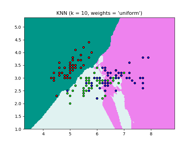
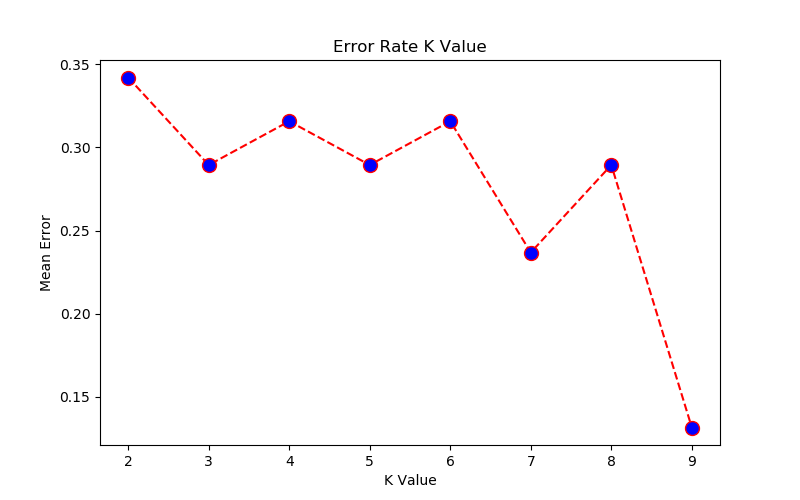
[x1, x2, x3 ... xm] are known values. [y1, y2 ... yp] are known labels. Equation of hyperplane is f(x) = xTβ + b = 0. Any classification task usually involves following steps:
- separate data into training and testing sets where each instance in the training set contains one target value or desired output (i.e. the class labels) and several attributes (i.e. the features or observed variables)
- produce a model (based only on the training data) which predicts the target values
- check the model on the test data given only the test data attributes
Support vector machines (SVM) were originally designed for binary (type-1 or type-2) classification. Some other methods known for multi-class classification are "one-against-all or one-vs-all", "one-against-one" and Directed Acyclic Graph Support Vector Machines (DAGSVM). SVM requires that each data set is represented as a vector of real numbers as shown below. Each column is known as class or category and each row is an observation (training data).
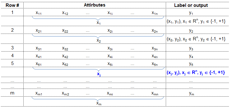
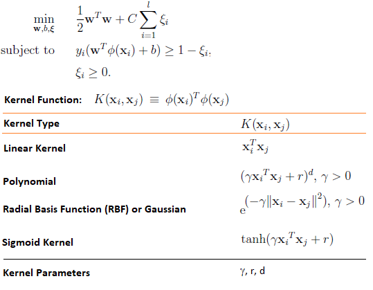
Reference: A Practical Guide to Support Vector Classfication by Chih-Wei Hsu, Chih-Chung Chang and Chih-Jen Lin, Department of Computer Science, National Taiwan University, Taipei 106, Taiwan
Scaling before applying SVM is very important. The main advantage of scaling is to avoid attributes in greater numeric ranges dominating those in smaller numeric ranges. Another advantage is to avoid numerical difficulties during the calculation. Because kernel values usually depend on the inner products of feature vectors, e.g. the linear kernel and the polynomial kernel, large attribute values might cause numerical problems. We recommend linearly scaling each attribute to the range [-1; +1] or [0; 1].
In general, the RBF kernel is a reasonable first choice. This kernel non-linearly maps samples into a higher dimensional space so it can handle the case when the relation between class labels and attributes is non-linear. If the number of features is large, one may not need to map data to a higher dimensional space. That is, the non-linear mapping does not improve the performance. Using the linear kernel is good enough, and one only searches for the parameter C.There are two parameters for an RBF kernel: C and γ. It is not known beforehand which C and γ are best for a given problem; consequently some kind of model selection (parameter search) must be done. The goal is to identify good (C, γ) so that the classifier can accurately predict unknown data (i.e. testing data). If the number of features is large, one may not need to map data to a higher dimensional space. That is, the non-linear mapping does not improve the performance. Using the linear kernel is good enough, and one only searches for the parameter C.
Support Vector Machines (clustering algorithm) tested for iris.data.
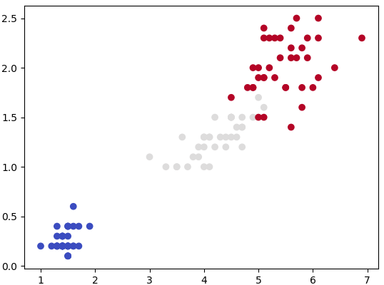
#        ssssssss       v           v       M            M
#        ss              v         v        M  M       M M
#        ss               v       v         M    M   M   M
#        ssssssss          v     v          M      M     M
#              ss           v   v           M            M
#              ss            v v            M            M
#        ssssssss             v             M            M
#
# SVM: "Support Vector Machine" (SVM) is a supervised ML algorithm which can be
#      used for both (multi-class) classification and/or (logistic) regression.
# Support vectors: vectors formed by observations w.r.t. origin
# Support Vector Machine is a separator which best segregates the two or more
# classes (hyperplanes or lines).

from sklearn import svm
import matplotlib.pyplot as plt
import numpy as np
import pandas as pd
#from sklearn import datasets     # Get pre-defined datasets e.g. iris dataset

# importing scikit learn with make_blobs
from sklearn.datasets.samples_generator import make_blobs

# creating datasets X containing n_samples, Y containing two classes
x, y = make_blobs(n_samples=500, centers=2, random_state=0, cluster_std=0.40)

#Generate scatter plot
#plt.scatter(x[:, 0], x[:, 1], c=y, s=50, cmap='spring')

'''
#------------------ Read the data ---------------------------------------------
dat = pd.read_csv("D:/Python/Abc.csv")
X = dat.drop('Class', axis=1)   #drop() method  drops the "Class" column
y = dat['Class']
'''
header=['sepal-length', 'sepal-width', 'petal-length', 'petal-width', 'Class']
df = pd.read_csv('iris.csv', names=header)
A = df.iloc[:, 2:4].values   # Use the last two features: note 2:4 slice
#To get columns C to E (unlike integer slicing, 'E' is included in the columns)
#df.loc[:, 'C':'E']

L = df.iloc[:, 4].values     # Labels: last column of input data

from sklearn.model_selection import train_test_split
X_trn, X_test, Y_trn, Y_test = train_test_split(A, L, test_size = 0.25)

#plt.scatter(x[:, 0], x[:, 1], c=y, s=50, cmap='spring')
plt.scatter(X_trn[:, 0], X_trn[:, 1], c=Y_trn, cmap=plt.cm.coolwarm)
plt.show()                         #By default, pyplot does not show the plots

#------------------ Specify SVM parameters ------------------------------------
# Specify penalty or regularization parameter 'C'
C = 1.0

# Carry out SVM calculation using kernel 'linear', 'rbf -  Gaussian kernel'
# 'poly', 'sigmoid'. Here rbf, poly -> non-linear hyper-planes
# rbf = Radial Basis Function Kernel
# gamma: Kernel coefficient for 'rbf', 'poly' and 'sigmoid'.
# Higher value of gamma tries to exact fit the training data -> over-fitting

# 'linear' -> classify linearly separable data
'''
from sklearn.svm import SVC
svcLin = SVC(kernel='linear', C=1, gamma='auto')
svcPoly = SVC(kernel='poly', degree=8)
svcc.fit(X_trn, Y_trn)
'''
# Following line of code is equivalent to the 3 short lines described above
svcLin1 = svm.SVC(kernel='linear', C=1.0, gamma='scale').fit(X_trn, Y_trn)
svcRBF = svm.SVC(kernel='rbf', C=1.0, gamma='scale').fit(X_trn, Y_trn)
svcPoly3 = svm.SVC(kernel='poly', C=1.0, degree=3).fit(X_trn, Y_trn)
svcLin2 = svm.LinearSVC(C=1.0, max_iter=10000).fit(X_trn, Y_trn)
# --------------- Create x-y grid to generate a plot --------------------------
#Calculate x- and y-limits
x_min, x_max = X_trn[:, 0].min() - 1, X_trn[:, 0].max() + 1
y_min, y_max = X_trn[:, 1].min() - 1, X_trn[:, 1].max() + 1
#Calculate grid size on x- and y-axis
h = (x_max - x_min)/100
xx, yy = np.meshgrid(np.arange(x_min, x_max, h), np.arange(y_min, y_max, h))

# ----------------- Generate the plot ------------------------------------------
# title for the plots
titles = ['SVC-No-Kernel', 'SVC-RBF', 'SVC-poly-3', 'LinearSVC']
for i, classifier in enumerate((svcLin1, svcRBF, svcPoly3, svcLin2)):
    # Plot the decision boundary and assign a color to each point
    plt.subplot(2, 2, i + 1)
    plt.subplots_adjust(wspace=0.4, hspace=0.4)

    #numpy.c_: Translates slice objects to concatenation along the second axis
    #numpy.ravel: returns a contiguous flattened array
    Z = classifier.predict(np.c_[xx.ravel(), yy.ravel()])

    #Put the result into a color plot
    Z = Z.reshape(xx.shape)
    plt.contourf(xx, yy, Z, cmap=plt.cm.gray, alpha=0.8)

    #Plot also the training points
    plt.scatter(X_trn[:,0], X_trn[:,1], c=Y_trn, facecolors='none', edgecolors='k')
    plt.xlabel('X1')
    plt.ylabel('X2')
    plt.xlim(xx.min(), xx.max())
    plt.ylim(yy.min(), yy.max())
    plt.xticks(())
    plt.yticks(())
    plt.title(titles[i])
plt.show()                        #By default, pyplot does not show the plots
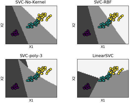
It is an unsupervised clustering algorithm where user needs to specify number of clusters - based on certain insights or even the "later purpose such as number of market segments". Though the number of clusters may not be known a-priori, a practically 'optimum' value can be estimated by "elbow method". It is a plot of cost function (grand total of distances between the cluster centroid and the observations) vs. number of clusters. Very often but not always, the curve looks like a "bent human hand" and the elbow represents the point where the curve has noticeable change in slope - the optimal value of 'K'.
- K-Means is also known as "hard clustering" technique where each input data point is associated with a unique cluster and thus lack flexibility in shape of clusters.
- There is no "probability function" or uncertainty associated with clustering to describe how close or appropriate this classification is.
- k-means inherently assumes that the cluster models must be circular and has no built-in way of accounting for oblong or elliptical clusters.
- Enhancements comes in the form of a GMM - Gaussian Mixture Model. Excerpt from scikit-learn: GMM is a probabilistic model that assumes all the data points are generated from a mixture of a finite number of Gaussian distributions with unknown parameters. This is a generalizing k-means clustering to incorporate information about the covariance structure of the data as well as the centers of the latent Gaussians.
- Thus, GMM is a 'soft' version of k-means.
# ----Ref: github.com/trekhleb/machine-learning-octave/tree/master/k-means-----
% K-means is an example of unsupervised learning, an iterative method over
% entire data. K-means is a clustering method and not classification method.
% Input is a set of unlabelled data and output from k-means is a set or sub-
% set of coherent data. It is not same as K-Nearest-Neighbours [KNN].
%
% Initialization
clear; close all; clc;

% ------------------------------ Clustering -----------------------------------
%Load the training data
load('set1.mat');

%Plot the data.
subplot(2, 2, 1);
plot(X(:, 1), X(:, 2), 'k+','LineWidth', 1, 'MarkerSize', 7);
title('Training Set');

%Train K-Means: The first step is to randomly initialize K centroids.
%Number of centroids: how many clusters are to be defined
K = 3;

%How many iterations needed to find optimal centroids positions 'mu'
max_iter = 100;
% Initialize some useful variables.
[m n] = size(X);

%Step-1: Generate random centroids based on training set. Randomly reorder the
%indices of examples: get a row vector containing a random permutation of 1:n
random_ids = randperm(size(X, 1));

% Take the first K randomly picked examples from training set as centroids
mu = X(random_ids(1:K), :);

%Run K-Means.
for i=1:max_iter
  % Step-2a: Find the closest mu for training examples.
  % Set m
  m = size(X, 1);

  % Set K
  K = size(mu, 1);

  % We need to return the following variables correctly.
  closest_centroids_ids = zeros(m, 1);

  %Go over every example, find its closest centroid, and store
  %the index inside closest_centroids_ids at the appropriate location.
  %Concretely, closest_centroids_ids(i) should contain the index of centroid
  %closest to example i. Hence, it should be a value in the range 1..K
  for i = 1:m
    d = zeros(K, 1);
    for j = 1:K
      d(j) = sum((X(i, :) - mu(j, :)) .^ 2);
    end
    [min_distance, mu_id] = min(d);
    closest_centroids_ids(i) = mu_id;
  end

  %Step-2b: Compute means based on closest centroids found in previous step
  [m n] = size(X);

  %Return the following variables correctly
  mu = zeros(K, n);

  %Go over every centroid and compute mean of all points that belong to it.
  %Concretely, the row vector centroids(i, :) should contain the mean of the
  %data points assigned to centroid i.
  for mu_id = 1:K
    mu(mu_id, :) = mean(X(closest_centroids_ids == mu_id, :));
  end
end

% Plotting clustered data
subplot(2, 2, 2);
for k=1:K
  % Plot the cluster - this is the input data marked as subsets or groups
  cluster_x = X(closest_centroids_ids == k, :);
  plot(cluster_x(:, 1), cluster_x(:, 2), '+');
  hold on;

  % Plot the centroid estimated by clustering algorithm
  centroid = mu(k, :);
  plot(centroid(:, 1), centroid(:, 2), 'ko', 'MarkerFaceColor', 'r');
  hold on;
end
title('Clustered Set');
hold off;
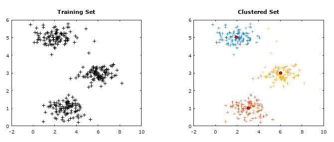
Machine Learning: Hierarchical Clustering
This type of clustering method is used on a relatively smaller datasets as the number of computation is proportional to N3 which is computationally expensive on big datasets and may not fit into memory.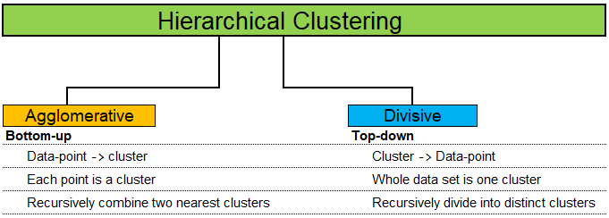
Random Forest Algorithm with Python and Scikit-Learn
Random Forest is a supervised method which can be used for regression and classification though it is mostly used for the later due to inherent limitations in the former. As a forest comprised of trees, a Random Forest method use multiple Decision Trees to arrive at the classification. Due to multiple trees, it is less prone to over-fitting and can handle relatively larger dataset having higher dimensionality (higher number of features). It is also known as Ensemble Machine Learning algorithm where many weak learning algorithms (the decision trees) are used to generate a majority vote (the stronger team). Bagging and boosting are two methods used in Random Forest learning algorithm to improve its performance: reduce bias and variance, increase accuracy.Bagging: bootstrap aggregation - where bootstring refers to training samples generated at random but with replacements. e.g. k samples out of N training data.Thus, the rows in each training samples may contain repeated values.
Boosting: it is an iterative approach by adjusting the probability of an instance to be part of subsequent training dataset if it is not correctly classified. The method starts with assigning equal probability to each instance to be part of first training set T1. The classifier C1 is trained on T1. It is then used to predict instances [xi, yi, i = 1, 2, 3 ... N]. If instances xm, xp and xz are not correctly classified, a higher probability will be assigned to these instances to be part on next training set T2. Since the selection of dataset is random, there are rows of dataset which may not make it to the any training set. They are known as out-of-bag dataset. A practically useful boosting algorithm is AdaBoost (which is a shorthand for Adaptive Boosting). The AdaBoost algorithm outputs a hypothesis that is a linear combination of simple hypotheses where an efficient weak learner is 'boosted' into an efficient strong learner.
Following example demonstrates use of Python and sciKit-Learn for classification. Problem Statement: The task here is to predict whether a person is likely to become diabetic or not based on four attributes: Glucose, Blood Pressure, BMI, Age.
The data in CSV format can be downloaded from here.import pandas as pd
import numpy as np
# --------- STEP-1: Read the dataset -------------------------------------------
dataset = pd.read_csv('diabetesRF.csv')
dataset.head()
X = dataset.iloc[:, 0:4].values
y = dataset.iloc[:, 4].values
# --------- STEP-2: Split the data into training and test sets -----------------
#Divide data into attributes and labels
from sklearn.model_selection import train_test_split
X_tr, X_ts, y_tr, y_ts = train_test_split(X, y, test_size=0.3, random_state=0)
#test_size: if float, should be between 0.0 and 1.0 and represents proportion
#of the dataset to include in the test split. If int, represents the absolute
#number of test samples. If 'None', the value is set to the complement of the
#train size. If train_size is also 'None', it will be set to 0.25.
# --------- STEP3: Scale the features ------------------------------------------
from sklearn.preprocessing import StandardScaler
sc = StandardScaler()
X_tr = sc.fit_transform(X_tr)
X_ts = sc.transform(X_ts)
# --------- STEP-4: Train the algorithm ----------------------------------------
from sklearn.ensemble import RandomForestClassifier
clf = RandomForestClassifier(n_estimators=20, random_state=0)
clf.fit(X_tr, y_tr)
y_pred = clf.predict(X_ts)
#
# --------- STEP-5: Evaluate the Algorithm -------------------------------------
from sklearn.metrics import classification_report, confusion_matrix
from sklearn.metrics import accuracy_score
#
#scikit-learn.org/stable/modules/generated/sklearn.metrics.confusion_matrix.html
#Compute confusion matrix to evaluate the accuracy of a classification. By
#definition a confusion matrix C is such that Cij is equal to the number of
#observations known to be in group 'i' but predicted to be in group 'j'. Thus
#in binary classification, the count of true negatives is C(0,0), false
#negatives is C(1,0), true positives is C(1,1) and false positives is C(0,1).
#
#In sciKit-learn: By definition, entry (i, j) in a confusion matrix is number of
#observations actually in group 'i', but predicted to be in group 'j'. Diagonal
#elements represent the number of points for which the predicted label is equal
#to the true label, while off-diagonal elements are those that are mislabeled by
#the classifier. Higher the diagonal values of the confusion matrix the better,
#indicating many correct predictions. i = 0, j = 0 -> TN, i = 0, j = 1 -> FP
#
print("Confusion Matrix as per sciKit-Learn")
print(" TN | FP ")
print("-------------------")
print(" FN | TP ")
print(confusion_matrix(y_ts,y_pred))
#
# Confusion matrix in other programs and examples
#
# Actual Values
# .----------------------,---------------------.
# P ! | !
# r Positives (1) ! True Positives (TP) | False Positives (FP)!
# e ! Predicted = Actual | (Type-1 Error) !
# d ! | !
# i !----------------------|---------------------!
# c ! | !
# t Negatives (0) ! False Negatives (FN)| True Negatives (TN) !
# e ! (Type-II Error) | Predicted = Actual !
# d ! | !
# Value !......................!.....................|
#
print("Classification Report format for BINARY classifications")
# P R F S
# Precision Recall fl-Score Support
# Negatives (0) TN/[TN+FN] TN/[TN+FP] 2RP/[R+P] size-0 = TN + FP
# Positives (1) TP/[TP+FP] TP/[TP+FN] 2RP/[R+P] size-1 = FN + TP
#
# F-Score = harmonic mean of precision and recall - also known as the Sorensen–
# Dice coefficient or Dice similarity coefficient (DSC).
# Support = class support size (number of elements in each class).
#
print(classification_report(y_ts, y_prd))
#
# Print accuracy of the classification = [TP + TN] / [TP+TN+FP+FN]
print("Classifier Accuracy = {0:8.4f}".format(accuracy_score(y_ts, y_prd)))
#
# --------- STEP-6: Refine the Algorithm ---------------------------------------
Recall: How many relevant items are selected?
Precision: How many selected items are relevant?
Decision Tree: This is a supervised classification method. Refer to the following decision making chart.
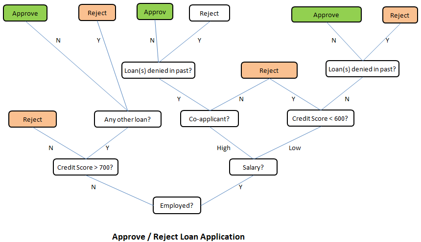

The method "decision tree" inherits this name from the structure of a 'tree' and the final intent to arrive at a 'decision' after going through a set of steps. As evident from the layout, the process starts with a "main node" known as "root node" and branches into other "leaf nodes" like a tree. In machine learning algorithms, following key points need to be addressed: Which attribute to select as root node? How to split attributes? When to stop? Before one gets to the answers, following concepts related to this machine learning methods needs to be understood:
- Entropy: This is a measure of impurity, uncertainty and information content. In thermodynamics and statistical mechanics, entropy is measure of disorder or randomness. In other words, entropy is a measure of lack of order. Entropy = Σ(-pi . log2pi). Entropy concepts have been adopted from information theory. The higher the entropy the more the information content or impurity.
- Information Gain: This is a measure of reduction in uncertainties and hence value lies between 0 and 1. Information gain tells us how important a given attribute of the feature vectors is and hence how useful it is for discriminating between the classes to be learned. Information gain = ENTROPYPARENT - average(ENTROPYCHILDREN).
- What is the entropy of a group in which all examples belong to the same class?
- A: pi = 1.0, Entropy = 0.0. This is not considered a good training set for learning.
- What is the entropy of a group with 50% in either class?
- A: pi = 0.5, Entropy = 1.0. This is considered a good training set for learning.
| Salaried | Married | Owns a house | Invests in Stocks? |
| Low | Y | 2BHK | 1 |
| Low | N | 2BHK | 1 |
| Low | Y | 3BHK | 0 |
| High | N | 3BHK | 0 |
p+ = fraction of positive examples = 2/4 = 0.5
p- = fraction of negative examples = 2/4 = 0.5
Thus: entropy of parent = Σ(-pi . log2pi) = -p+ log2(p+) - p- log2(p-) = 1.0.Split on feature 'Salaried'
| Salaried | Invests in Stocks? |
| Low | 1 |
| Low | 1 |
| Low | 0 |
| High | 0 |
Similarly, there is 1 instance of 'High' resulting in 1 negative label (class). p+,HIGH = 0. Hence, p-, HIGH = 1 - 0 = 1. Entropy at child node: EHIGH = -p+, HIGH log2(p+, HIGH) - p-, HIGH log2(p-, HIGH) = -0 × log2(0) - 1 × log2(1) = 0.
Information gain = EPARENT - pLOW × ELOW - pHIGH × EHIGH = 1.0 - 3/4 × (log23 - 2/3) - 1/4 × 0 = 1.5 - 3/4×log2(3) =0.3112.Split on feature 'Married'
| Married | Invests in Stocks? |
| Y | 1 |
| N | 1 |
| Y | 0 |
| N | 0 |
Similarly, there are 2 instances of 'N' resulting in 1 positive label (class) and 1 negative class. p+,N = 1/2. Hence, p-, N = 1.0 - 1/2 = 1/2. Entropy at child node: EN = -p+, N log2(p+, N) - p-, N log2(p-, N) = -1/2 × log2(1/2) - 1/2 × log2(1/2) = 1.0.
Information gain = EPARENT - pY × EY - pN × EN = 1.0 - 2/4 × 1.0 - 2/4 × 1.0 = 0.0.Split on feature "Owns a House"
| Owns a House | Invests in Stocks? |
| 2BHK | 1 |
| 2BHK | 1 |
| 3BHK | 0 |
| 3BHK | 0 |
Similarly, there are 2 instances of '3BHK' resulting in 2 negative label (class). p-,3HBK = 2/2 = 1.0. Hence, p+, 3BHK = 1.0 - 1.0 = 0.0. Entropy at child node: E3BHK = -p+, 3BHK log2(p+, 3BHK) - p-, 3BHK log2(p-, 3BHK) = -0.0 × log2(0.0) - 1.0 × log2(1.0) = 0.0.
Information gain = EPARENT - p2BHK × E2BHK - p3BHK × E3BHK = 1.0 - 2/4 × 0.0 - 2/4 × 0.0 = 1.0.Thus splitting on attribute (feature) "Owns a House" is best.
Probability in Machine Learning
Bayes theorem is a basis of a popular algorithm known as Naive Bayes Classification. This is widely used in text filtering such as classification of an e-mail as genuine or spam, categorization of a news article or user comment as fair or abusing / derogatory and the famous Monty Hall problem. However, it gets a bit complicated as the term 'odds' is also used to express the likelihood of an event - where 'odds' is not same as 'probability'. The odds of an event [E] vs. event "not E" or event [E'] are the ratio of their probabilities. For a standard dice, the odds of rolling digit 3 is [1/6] / [5/6] = 1:5, that the odds are "1 to 5 for" or "5 to 1 against" rolling a 3. The adjective 'Naive' refers to the "Naive assumption" of conditional independence between every pair of a feature.Bayes theorem is based on conditional probability that is based on some background (prior) information. For example, every year approximately 75 districts in India faces drought situation. There are 725 districts in India. Thus, the probability that any randomly chosen district will face rain deficit in next year is 75/725 = 10.3%. This value when expressed as ratio will be termed prior odds. However, there are other geological factors that governs the rainfall and the chances of actual deficit in rainfall may be higher or lower than the national average.
Suppose section A of class 8 has 13 boys and 21 girls. Section B of the same class has 18 boys and 11 girls. You randomly calls a student by selecting a section randomly and it turns out to be a girl. What is the probability that the girl is from section A? Let:
- H = event that the student selected is from section 'A'
- G = event that the student selected is a 'girl'
- In terms of conditional probability (it is already known that the student picked is a girl), p(H|G) refers to the probability that the event 'H' occurred given that 'G' is known to have occurred. There is no straightforward way to estimate this value!
- However, it is very easy to calculate the the probability of student picked to be a girl if it is known that section chosen is A. That is, p(G|H) = 21/34.
- Bayes theorem is used to estimate p(H|G). Here p(H|G) = p(H)/p(G) × p(G|H). Thus, p(H/G) = [1/2] / [33/63] × 21/34 = 11/68.
- prior probability = p(H) = probability of the hypothesis before we see the data (girl being picked)
- posterior probability = p(H|G) = probability of the hypothesis (girl is from section A) after we see the data (girl is being picked) and the the value one is interested to compute.
- p(G|H) = probability of the data (girl) under the hypothesis (section A), called the likelihood.
In english translation, the meaning or synonyms of 'odds' are 'chances', 'probability', 'likelyhood'. However, 'odds' is distinguished from probability in the sense that the former is always a ratio of two integers where the later is a fraction which can be represented in %. By odds, for example 3:2 (three to 2), we convey that we expect that for every three cases of an outcome (such as a profitable trade), there are two cases of the opposite outcome (not a profitable trade). In other words, chances of a profitable trade are 3/[3+2] = 3/5 or probability of 60%.
If the metrological department of the country announces that it is 80% probability of a normal monsoon this year and it turns out to be a drought. Can we conclude that the weather forecast was wrong. No! The forecast said it is going to be a normal monsoon with 80% probability, which means it may turn out to be drought with 10% probability or 1 out of 5 years. This year turned out to be the 1 in 5 event. Can we conclude that the probability 80% was correct? No! By the same argument one could conclude that 75% chance of normal monsoon was also correct and both cannot be true at the same time.Likelihood ratio: The ratio used in example above (4 times higher chance of normal monsoon than not a normal monsoon) is called the likelihood ratio. In other words, likelihood ratio is the probability of the observation in case the event of interest (normal monsoon), divided by the probability of the observation in case of no event (drought). The Bayes rule for converting prior odds into posterior odds is:
posterior odds = likelihood ratio × prior odds or posterior odds = Bayes factor × prior odds.
- If "likelihood ratio" > 1, the posterior odds are greater than the prior odds and the data provides evidence in favour of hypothesis.
- If "likelihood ratio" < 1, the posterior odds are smaller than the prior odds and the data provides evidence against the hypothesis.
- If "likelihood ratio" = 1, the posterior odds are greater than the prior odds and the data provides evidence in favour of hypothesis.
Gaussian Naive Bayes on iris data using Python and scikit-learn
# --------------------------------- --------------------------------------------
# --- Gaussian Naive Bayes on IRIS data,  print confusion matrix as Heat Map ---

import numpy as np
import matplotlib
import matplotlib.pyplot as plt

#There are many built-in data sets. E.g. breast_cancer, iris flower type
#from sklearn.datasets import load_breast_cancer

#Load the iris dataset which is built into scikit-learn
from sklearn.datasets import load_iris
iris = load_iris()

#This object is  a dictionary and contains a description, features and targets:
#print(iris.keys())
#dict_keys(['target','target_names','data','feature_names','DESCR','filename'])

#Split matrix [iris] into feature matrix [X] and response vector {y}
X = iris.data           # X = iris['data'] - access data by key name
y = iris.target         # y = iris['target']

A = iris.target_names   # A = iris['target_names']
#print(A)
#['setosa' 'versicolor' 'virginica']

F = iris.feature_names  # F = iris['feature_names']
#print(F)
#['sepal length (cm)', 'sepal width (cm)', 'petal length (cm)', 'petal width (cm)']

L = np.array(['Label'])
#print(np.r_[[np.r_[F, L], np.c_[X, y]]])

#Split X and y into training and testing sets
from sklearn.model_selection import train_test_split
X_trn,X_test, y_trn,y_test = train_test_split(X,y, test_size=0.4,random_state=1)

#Train the model on training set
from sklearn.naive_bayes import GaussianNB
gnb = GaussianNB()
clf = gnb.fit(X_trn, y_trn)

#Make predictions on test data
y_pred = gnb.predict(X_test)

#Compare actual response values (y_test) with predicted response values (y_pred)
from sklearn import metrics
from sklearn.metrics import classification_report, confusion_matrix
from sklearn.metrics import accuracy_score

GNBmetric = metrics.accuracy_score(y_test, y_pred)*100
print("Gaussian Naive Bayes model accuracy (in %): {0:8.1f}".format(GNBmetric))

#2D list or array which defines the data to color code in Heat Map
XY = confusion_matrix(y_test, y_pred)
print(XY)

fig, ax = plt.subplots()
#The heatmap is an imshow plot with the labels set to categories defined by user
from matplotlib.colors import ListedColormap
clr = ListedColormap(['red', 'yellow', 'green'])
im = ax.imshow(XY, cmap=clr)

#Define tick marks which are just the ascending integer numbers
ax.set_xticks(np.arange(len(A)))
ax.set_yticks(np.arange(len(A)))

#Ticklabels are the labels to show - the target_names of iris data = vector {A}
ax.set_xticklabels(iris.target_names)
ax.set_yticklabels(iris.target_names)

#Rotate the tick labels and set their alignment.
plt.setp(ax.get_xticklabels(), rotation=45, ha="right", rotation_mode="anchor")

#Loop over the entries in confusion matrix [XY] and create text annotations
for i in range(len(A)):
    for j in range(len(A)):
        text = ax.text(j, i, XY[i, j], ha="center", va="center", color="w")

ax.set_title("Naive Bayes: Confusion Matrix as Heat Map")
fig.tight_layout()
plt.show()
This generates the following plot. 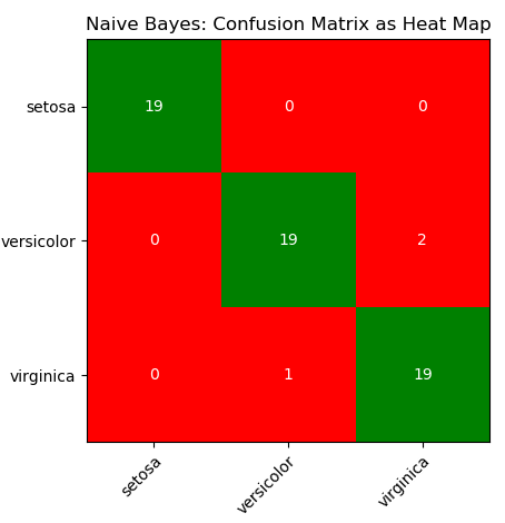
Monty-Hall Problem
Assume that in a TV show the candidate is given the choice between three doors. Behind two of the doors there is a pencil and behind one there is the grand prize, a car. The candidate chooses one door. After that, the show master opens another door behind which there is a pencil. Should the candidate switch doors after that? What is the probability of winning the car?Credibility of an Eyewitness
Assume that an eyewitness is 90% certain that a given person was involved in an accident. Moreover, assume that there were 20 people around the parking lot at the time of the crime. What is the posterior probability of the person actually have committed the crime?ANN: Artificial Neural Network
Multi-Layer Perceptron is a supervised learning algorithm which can learn a non-linear function approximator for either classification or regression. It differs from a logistic regression algorithm in construction where between the input and the output layer, there are one or more non-linear (hidden) layers. The simplest neural network consists of only one neuron and is called a perceptron. The perceptron is simply a witty name for the simple neuron model with the step activation function. A method for learning the weights of the perceptron from data called the Perceptron algorithm was introduced by the psychologist Frank Rosenblatt in 1957. It is just about as simple as the nearest neighbor classifier. The basic principle is to feed the network training data one example at a time. Each incorrect classification leads to an update in the weights and biases.In scikit-learn, MLP is implemented as following classes:
- MLPRegressor: this is a multi-layer perceptron (MLP) class that trains using back-propagation with no activation function in the output layer, which can also be seen as using the identity function as activation function. It uses the sum of square error (SSE) as the loss function and generates output as continuous values.
- MLPClassifier: a multi-layer perceptron (MLP) algorithm that trains using back-propagation that is using some form of gradient descent and the gradients are calculated using back-propagation.
- Many types of activation functions are available such as step function, sigmoid function, relu function and tanh function. In general, (rectified linear unit) ReLU function is used in the hidden layer neurons and sigmoid function is used for the output layer neuron.
Tensors
Tensors are a generalization of matrices. A constant or scalar is 0-dimensional tensor, a vector is a 1-dimensional tensor, a 2×2 matrix is a 2-dimensional tensor, a 3×3 matrix is a 3-dimensional tensor and so on. The fundamental data structure for neural networks are tensors. In summary, arrays, vectors, matrices and tensors are closely related concepts and differ only in the dimensions. All of these are a representation of a set of data with indices to locate and retrieve them.Steps to create a simple artificial neural network (ANN)
- Step-0: Read the data and manipulate it as per requirements of machine learning algorithms. For example, the labels may be categorical such as 'Rare', 'Low', 'Medium', 'High'. Neural networks (and most machine learning algorithms) work better with numerical data [0, 1, 2...]. Convert the categorical values to numerical values using LabelEncoder class from scikit-learn. Use y.Class.unique() to find unique categories in label vector.
- Step-1: Define the input layer, hidden layer(s) and the output layer. Chose activation function for every hidden layer - Sigmoid activation function is the most widely used one. Multi-layer Perceptron is sensitive to feature scaling, so it is highly recommended to scale the data - StandardScaler from scikit-learn can be used for standardization.
- Step-2: Feedforward or forward propagation: assumed weights [W] and biases [b] and calculate the predicted output y. Estimate accuracy of predictions using a Loss Function such as sum of squares error (SSE).
- Step-3: Back propagation: adjust weights and biases and calculate the predicted output y using gradient decent method which is based on derivative of the loss function with respect to the weights and biases.
- Step-4: Train the model
- Step-5: Test the model
# -------------------------------- ---------------------------------------------
# --- ANN - Multi-layer Perceptron,  print confusion matrix as Heat Map ---
import numpy as np
import matplotlib
import matplotlib.pyplot as plt

#There are many built-in data sets. E.g. breast_cancer, iris flower type
#from sklearn.datasets import load_breast_cancer
#df = load_breast_cancer()

#Load the iris dataset which is built into scikit-learn
from sklearn.datasets import load_iris
df = load_iris()

#This object is  a dictionary and contains a description, features and targets:
#print(df.keys())
#dict_keys(['target','target_names','data','feature_names','DESCR','filename'])

#Split matrix [df] into feature matrix [X] and response vector {y}
X = df.data           # X = df['data'] - access data by key name
y = df.target         # y = df['target']

A = df.target_names   # A = df['target_names']
#print(A)
#['setosa' 'versicolor' 'virginica']

F = df.feature_names  # F = df['feature_names']
#print(F)
#['sepal length (cm)', 'sepal width (cm)', 'petal length (cm)', 'petal width (cm)']

L = np.array(['Label'])
#print(np.r_[[np.r_[F, L], np.c_[X, y]]])

# splitting X and y into training and testing sets
from sklearn.model_selection import train_test_split
X_trn,X_test, y_trn,y_test = train_test_split(X,y, test_size=0.4,random_state=1)

#Scale or normalize the data
from sklearn.preprocessing import StandardScaler
#StandardScaler(copy=True, with_mean=True, with_std=True)
scaleDF = StandardScaler()
#Fit to the training data
scaleDF.fit(X_trn)
#Apply transformations to the data
X_trn = scaleDF.transform(X_trn)
X_test = scaleDF.transform(X_test)

#Train the model on training set
from sklearn.neural_network import MLPClassifier
ann_mlp = MLPClassifier(solver='lbfgs', alpha=1e-5,
                        hidden_layer_sizes=(5, 3), random_state=1)
clf = ann_mlp.fit(X_trn, y_trn)

#hidden_layer_sizes=(5, 3) - two layers having 5 and 3 nodes each
#max_iter = number of cycle of "feed-forward and back propagation" phase.

#Make predictions on the testing set
y_pred = ann_mlp.predict(X_test)

#Compare actual response (y_test) with predicted response (y_pred)
from sklearn import metrics
from sklearn.metrics import classification_report, confusion_matrix
from sklearn.metrics import accuracy_score

MLPmetric = metrics.accuracy_score(y_test, y_pred)*100
print("MLP accuracy(in %): {0:8.1f}".format(MLPmetric))

#2D list or array which defines the data to color code in Heat Map
XY = confusion_matrix(y_test, y_pred)
print(XY)
print(classification_report(y_test, y_pred))

fig, ax = plt.subplots()
#The heatmap is an imshow plot with the labels set to categories defined by user
from matplotlib.colors import ListedColormap
clr = ListedColormap(['grey', 'yellow', 'green'])
im = ax.imshow(XY, cmap=clr)

#Define the tick marks which are just the ascending integer numbers
ax.set_xticks(np.arange(len(A)))
ax.set_yticks(np.arange(len(A)))

#ticklabels are the labels to show - the target_names of iris data = vector {A}
ax.set_xticklabels(df.target_names)
ax.set_yticklabels(df.target_names)

#Rotate the tick labels and set their alignment.
plt.setp(ax.get_xticklabels(), rotation=45, ha="right", rotation_mode="anchor")

#Loop over the entries in confusion matrix [XY] and create text annotations
for i in range(len(A)):
    for j in range(len(A)):
        text = ax.text(j, i, XY[i, j], ha="center", va="center", color="w")

ax.set_title("ANN - Multi-layer Perceptron: Confusion Matrix")
fig.tight_layout()
plt.show()
Output of the program - MLP accuracy(in %): 70.0. Note that the lesser accuracy generated by the program does not highlight any deficiency in the algorithm or solver. This is only to show that there is no unique way of chosing the ANN parameters and optimal values need to be worked out by trial-and-error.
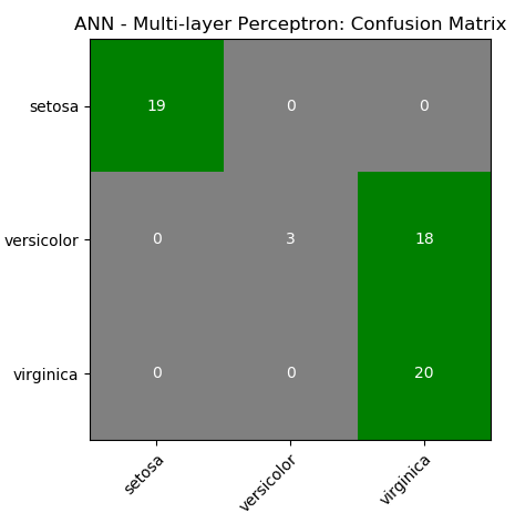
CNN
Convolutional Neural Networks (ConvNet or CNN) are special type of neural networks that handle image understanding and classification tasks by operating directly on the pixel intensities of input images. Thus, there is no need to explicitly perform any feature extraction operation.Digit Recognition
Excerpts from MathWorks Inc: "Object classification is an important task in many computer vision applications, including surveillance, automotive safety, and image retrieval. For example, in an automotive safety application, you may need to classify nearby objects as pedestrians or vehicles." The hand-written characters come in various shapes, size and colour. The correct classification of digits is one of the key aspects or capabilities of any ANN algorithm. This section describes the ANN implemented in MATLAB or GNU OCTAVE. The process starts with a dataset of digits (MNIST database or any similar ones) stored in this CSV file in Zip format.The information contained therein can be visualized using following script.
% ------ Handwritten digits classification ------------------------------------
%clear;
close all; clc;
colormap(gray);  % Use gray image colourmap
%
% Every row in X is a squared image reshaped into vector, width of each image
% is square root of total number of columns - 1 . The last column represents
% the actual digit hidden in those pictures. There are 500 examples each of 0,
% 1, 2, 3 ... 9.

A = csvread("digits.csv");
X =  A(:, 1:end-1);          %All columns except last one are pixels
Y = A(:, end);               %Last column has labels: 10 for digit '0'

% Randomly select N data points: required to split the dataset into training
% and test data. If N > 1, it is number. If it is a fraction, it is % of total
N_trn = 3000;
%
m = size(X, 1);        %Number of rows of X = no. of digits stored in  dataset
n = size(X, 2);        %Number of columns of X
nP = round(sqrt(n));   %Number of pixels rows,columns to represent each digit

% First row:
%   * * * * *  @ @ @ @ @  # # # # #      ```      $ $ $ $ $  [1 x n] vector
%
%   * * * * *
%   @ @ @ @ @
%   # # # # #
%      ...
%   $ $ $ $ $
%   D(1) = [nP x nP] matrix

% Second row:
%   * * * * *  @ @ @ @ @  # # # # #      ```      $ $ $ $ $  [1 x n] vector
%
%   * * * * *
%   @ @ @ @ @
%   # # # # #
%      ...
%   $ $ $ $ $
%   D(2) = [nP x nP] matrix

%Set padding: gap (shown as black background) between two consecutive images
pad = 2; ii = 25; jj = 20;
iR = pad + ii * (nP + pad);
iC = pad + jj * (nP + pad);
digit = -ones(iR, iC);

for s = 1: 10
% Copy each example into a [nP x nP] square block in the display array digit()
for i = 1:ii
 k = (i-1)*jj + 1 + (s-1)*ii*jj;
 for j = 1:jj
  % Get the max value of current row
  max_val = max(abs(X(k, :)));

  dR = pad + (i - 1) * (nP + pad) + (1:nP);
  dC = pad + (j - 1) * (nP + pad) + (1:nP);

  digit(dR, dC) = reshape(X(k, :), nP, nP) / max_val;
  k = k + 1;
 end
end

%imagesc(img) = display a scaled version of the matrix 'img' as a color image
%Colormap is scaled so that entries of the matrix occupy the entire colormap.
h = imagesc(digit, [-1 1]);    % Display Image
axis image off;        % Do not show axes

% Update figure windows and their children. Only figures that are modified
% will be updated. The refresh function can also be used to cause an update of
% the current figure, even if it is not modified.
drawnow;
str = sprintf(num2str(s-1));
saveas(h, str, 'png');

end
Rasterize and Vectorize: these are two frequently occuring terms in image handling programs. 'Rasterize' refers to converting an objects / images into pixels (though it is counter-intuitive as images are stored as pixels). Vectorization is a process of converting pixel information into geometry or outline information. The difference can be easily understood when texts are stored as 'non-selectable' images in a PDF (raster form) and same text are stored as 'selectable' objects in a PDF document (vector form).
Raster images lose quality when scaled up, resulting in pixelation (stair-stepping) and blurriness. Vector graphics consist of geometric shapes such as Bezier curves, B-splines, NURBS, arcs and lines determined by mathematical equations. Vector images can be significantly scaled without losing quality and hence such graphics are most appropriate for logos, icons, maps, graphs, illustrations... Vector images often result in smaller file sizes than raster images. Glyph Conversion is the method where tools like MS-Word translates the text characters into their corresponding visual glyphs (the shapes of the letters) based on font type. This makes the display theoretically "infinitely scalable". As the same time, it is counter-intuitive to think that when computer displays consists of finite number of pixels, how texts in MS-Word can be zoomed 'infinitely' without any stair-stepping? In real-life, one cannot draw a curve with smooth edge using small squares of uniform and finite size?
The images generated for digits 0, 3, 5 and 8 are shown below. The images for digit '1', digit '2', digit '3', digit '4', digit '5', digit '6', digit '7', digit '8' and digit '9' are under the respective hyperlinks.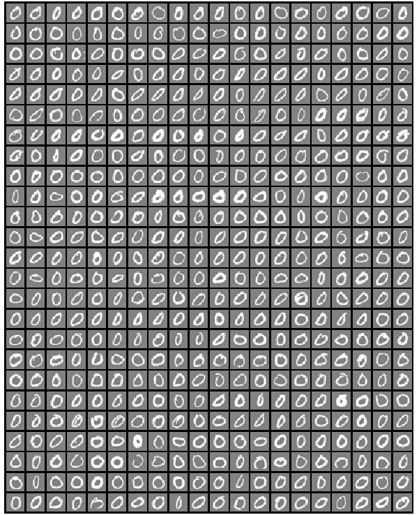
% ------ Handwritten digits classification -------------------------------------
clear; close all; clc;

%Load training data, display randomly selected 100 data: X is the input matrix
load('digits.mat');
[m n] = size(X);   %Matrix [5000, 400], 1-500: 0, 501-1000: 1, 1001-1500: 2....

%Create random permutation: a column vector of size = size of input [X]
random_digits_indices = randperm(m);

%Select first 100 entries from the random permutation generated earlier
random_digits_indices = random_digits_indices(1:100);

%Display the 100 images stored in 100 rows as [10x10] layout of digits
%display_data(X(random_digits_indices, :));

% Setup the parameters you will use for this part of the exercise
% Specify number of input images of digits.
nD = 30;
input_layer_size = nD*nD;

% 1 <= Number of labels of digits =< 10, (note "0" mapped to label 10)
num_labels = 10;

fprintf('Training One-vs-All Logistic Regression...\n')
lambda = 0.01;
n_iter = 50;  %try 50, 100, 200 and check training set accuracy

% Train the model and predict theta [q] - the label 0 to 9
[all_theta] = one_vs_all_train(X, y, num_labels, lambda, n_iter);

fprintf('Predict for One-Vs-All...\n')
[iR iC] = size(X);
accu = ones(num_labels, 1);
for i = 1: num_labels
  if (i == 10)
   pred = one_vs_all_predict(all_theta, X(1:500, :));
   accu(i) = mean(double(pred == y(1:500))) * 100;
   fprintf('\n Training accuracy for digit 0 = %5.2f [%%]\n', accu(i));
  else
   j = i * iR/10 + 1;
   k = (i+1) * iR/10;
   pred = one_vs_all_predict(all_theta, X(j:k, :));
   accu(i) = mean(double(pred == y(j:k))) * 100;
   fprintf('\n Training accuracy for digit %d = %5.2f [%%]', i, accu(i));
  endif
end
%pred = one_vs_all_predict(all_theta, X);
fprintf('\n Overall training accuracy for all digits: %5.2f [%%]\n', mean(accu));
Output:
Training One-vs-All Logistic Regression...
Iteration    50 | Cost: 1.308000e-02
Iteration    50 | Cost: 5.430655e-02
Iteration    50 | Cost: 6.180966e-02
Iteration    50 | Cost: 3.590961e-02
Iteration    50 | Cost: 5.840313e-02
Iteration    50 | Cost: 1.669806e-02
Iteration    50 | Cost: 3.502962e-02
Iteration    50 | Cost: 8.498925e-02
Iteration    50 | Cost: 8.042173e-02
Iteration    50 | Cost: 6.046901e-03
Predict for One-Vs-All...

Training accuracy for digit 1 = 98.40 [%]
Training accuracy for digit 2 = 93.20 [%]
Training accuracy for digit 3 = 91.80 [%]
Training accuracy for digit 4 = 96.00 [%]
Training accuracy for digit 5 = 91.80 [%]
Training accuracy for digit 6 = 98.40 [%]
Training accuracy for digit 7 = 95.20 [%]
Training accuracy for digit 8 = 92.40 [%]
Training accuracy for digit 9 = 92.60 [%]
Training accuracy for digit 0 = 99.80 [%]

Oaverall training accuracy for all digits: 94.96 [%]
%-------------- FUNCTION: one_vs_all_train --------------------------------
% Trains logistic regression model each of which recognizes specific number
% starting from 0 to 9. Trains multiple logistic regression classifiers and
% returns all the classifiers in a matrix all_theta, where the i-th row of
% all_theta corresponds to the classifier for label i.

function [all_theta] = one_vs_all_train(X, y, num_labels, lambda, num_iter)

  [m n] = size(X);
  all_theta = zeros(num_labels, n + 1);

  % Add column of ones to the X data matrix.
  X = [ones(m, 1) X];

  for class_index = 1:num_labels
   % Convert scalar y to vector with related bit being set to 1.
   y_vector = (y == class_index);

   % Set options for fminunc
   options = optimset('GradObj', 'on', 'MaxIter', num_iter);

   % Set initial thetas to zeros.
   q0 = zeros(n + 1, 1);

   % Train the model for current class.
   gradient_function = @(t) gradient_callback(X, y_vector, t, lambda);

   [theta] = fmincg(gradient_function, q0, options);

   % Add theta for current class to the list of thetas.
   theta = theta';
   all_theta(class_index, :) = theta;
  end
end
% ------ Testing: Make predictions with new images ----------------------------
% Predicts the digit based on one-vs-all logistic regression approach.
% Predict the label for a trained one-vs-all classifier. The labels
% are in the range 1..K, where K = size(all_theta, 1)
function p = one_vs_all_predict(all_theta, X)
  m = size(X, 1); num_labels = size(all_theta, 1);

  % We need to return the following variables correctly.
  p = zeros(m, 1);

  % Add ones to the X data matrix
  X = [ones(m, 1) X];

  % Calculate probabilities of each number for each input example.
  % Each row relates to the input image and each column is a probability that
  % this example is 1 or 2 or 3...
  z = X * all_theta';
  h = 1 ./ (1 + exp(-z));

  %Now let's find the highest predicted probability for each row: 'p_val'.
  %Also find out the row index 'p' with highest probability since the index
  %is the number we're trying to predict. The MAX utility is describe below.

  %For a vector argument, return the maximum value.  For a matrix argument,
  %return a row vector with the maximum value of each column. max (max (X))
  %returns the largest element of the 2-D matrix X.  If the optional third
  %argument DIM is present then operate along this dimension.  In this case
  %the second argument is ignored and should be set to the empty matrix. If
  %called with one input and two output arguments, 'max' also returns the
  %first index of the maximum value(s).  [x, ix] = max ([1, 3, 5, 2, 5])
  %  x = 5, ix = 3

  [p_vals, p] = max(h, [], 2);
end
Limitations of this script in its current format and structure:
- Any input image has to be in a row format of size [1 x 400] only.
- The image has to be in grayscale and exactly of size 20px × 20px only
- The intensities of pixels must be supplied as signed double precision numbers.
- The background of images has to be dark (black) or gray only with font in white colour. The images with white background and black font will not get recognized.
- The scale of pixel intensities has no unique upper and lower bounds. In the entire dataset, the lowest and the highest values are -0.13196 and 10.0 respectively.
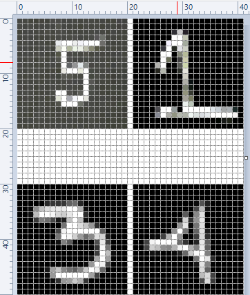
%Predict one digit at a time: digit from new set
fprintf('-----------------------------------------------------------------\n');
digit = 5; filename = [num2str(digit), ".png"];
dgt = rgb2gray(imread(filename));
Z = vec(im2double(dgt), 2);
%vec: return vector obtained by stacking the columns of the matrix X one above
%other. Without dim this is equivalent to X(:). If dim is supplied, dimensions
%of Z are set to dim with all elements along last dimension. This is equivalent
% to shiftdim(X(:), 1-dim).

pred = one_vs_all_predict(all_theta, Z);
fprintf('\nInput digit = %d, predicted digit = %d \n', digit, pred);
Input digit = 1, predicted digit = 5
Input digit = 3, predicted digit = 3Input digit = 4, predicted digit = 4
Input digit = 5, predicted digit = 3%------------------------------------------------------------------------------
Running the program repeatedly, correct prediction for digit 5 was obtained. However, the prediction for digit 1 remained as 5!
Further improvisation is possible by writing the answer on the right hand side or bottom of the image. Image is a matrix indexed by row and column values. The plotting system is, however, based on the traditional (x y) system. To minimize the difference between the two systems Octave places the origin of the coordinate system in the point corresponding to the pixel at (1; 1). So, to plot points given by row and column values on top of an image, one should simply call plot with the column values as the first argument and the row values as the second argument.%----------------- Example of PLOT over an IMAGE ------------------------------
I = rand (20, 20); %Generate a 2D matrix of random numbers
[nR, nC] = find (I > 0.95); %Find intensities greater than 0.95
hold ("on"); imshow (I); %Show image
plot(nC,nR,"ro"); hold ("off"); %Plot over the image
The output will look like: 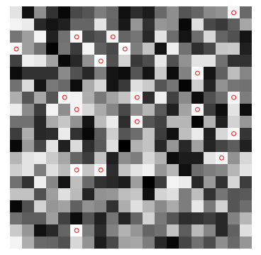
Digit Classification in Python
# --- Random Forest Classifier for Hand-written Digits ---

import matplotlib.pyplot as plt
from sklearn.datasets import load_digits
import pylab as pl

#Load hand-written digits from scikit-learn built-in database
digits = load_digits()

#Use a grayscale image
#pl.gray()
#pl.matshow(digits.images[0])
#pl.show()
#Check how digits are stored
print("Total digits in dataset are ", len(digits.images))

#Visualize few images in n x n matrix
n = 10
df = list(zip(digits.images, digits.target))
plt.figure(figsize = [5, 5])
for index, (image, label) in enumerate(df[:n*n]):
    plt.subplot(n, n, index+1)
    plt.axis('off')
    plt.imshow(image, cmap=plt.cm.gray_r, interpolation='nearest')
    #plt.title('%i' % label)
plt.show()

import random
from sklearn import ensemble, metrics
from sklearn.metrics import classification_report, confusion_matrix
from sklearn.metrics import accuracy_score

#Find out the number of digits, store label as variable y
nTest = len(digits.images)
x = digits.images.reshape(nTest, -1)
y = digits.target

#Create random indices to select training images, f = training set fraction
#The method used here is a longer version of train_test_split utility in sklearn
f = 0.20
idxTrain = random.sample(range(len(x)), round(len(x) * f))
idxTest = [i for i in range(len(x)) if i not in idxTrain]

#Sample and validation images
imgTrain = [x[i] for i in idxTrain]
imgTest = [x[i] for i in idxTest]

#Sample and validation targets
yTrain = [y[i] for i in idxTrain]
yTest = [y[i] for i in idxTest]

#Call random forest classifier
clf = ensemble.RandomForestClassifier(n_estimators=20, random_state=0)

#Fit model with training data
clf.fit(imgTrain, yTrain)

#Test classifier using validation images
score = clf.score(imgTest, yTest)
print("Random Forest Classifier: trained on ", len(imgTrain), "samples")
print("Score = {0:8.4f}". format(score))
#
yPred = clf.predict(imgTest)
XY = confusion_matrix(yTest, yPred)
print(XY)
Outputs from this Python code are:
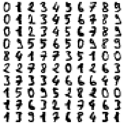
Total digits in dataset are  1797
Random Forest Classifier: trained on  359 samples
Score =   0.9075
[[138   0   0   0   2   0   1   0   1   0]
 [  0 134   0   1   0   1   0   0   1   5]
 [  1   3 127   6   1   0   1   0   3   1]
 [  0   1   5 127   0   0   0   2  10   3]
 [  3   2   0   0 141   1   1   4   0   0]
 [  1   0   0   3   0 128   1   1   0   5]
 [  1   1   0   0   2   0 141   0   0   0]
 [  0   0   0   0   1   1   0 136   1   0]
 [  0   9   3   2   0   2   2   3 117   0]
 [  0   2   0   7   2   5   1  12   5 116]]
CBIR: Content Based Image Retrieval systems: method to find similar images to a query image among an image dataset. Example CBIR system is the search of similar images in Google search. Convolutional denoising autoencoder [feed forward neural network] - class of unsupervised deep learning.
Computer Vision: OpenCV
Image processing is an integral part of computer vision. OpenCV (Open-source Computer Vision Library) is an open source computer vision and machine learning software library. It integrates itself seamlessly with Python and NumPy. In can be installed in Python 3.5 for Windows by command: C:\Windows\System32>py.exe -m pip install -U opencv-python. One can check the version by statement "print(cv2.__version__)" in Python. Python also has a library for image processing called 'Pillow'. Big difference between skimage imread and opencv is that it reads images as BGR instead of RGB (skimage). This link: github.com/BhanuPrakashNani/Image_Processing contains a detailed list (approx 35) of image processing methods and Python codes.- cv2.IMREAD_COLOR: Loads a color image. Any transparency of image will be neglected. It is the default flag. Same as cv2.imread("image_01.png", 1)
- cv2.IMREAD_GRAYSCALE: Loads image in grayscale mode, same as cv2.imread("image_01.png", 0)
- cv2.IMREAD_UNCHANGED: Loads image as such including alpha channel, same as cv2.imread("image_01.png", -1)
- Instead of these three flags, you can simply pass integers 1, 0 or -1 respectively as shown above
- OpenCV and skimage directly store imported images as numpy arrays
- Maintain output window until user presses a key or 1000 ms (1s): cv2.waitKey(1). cv2.waitKey(0) display the window until any key is pressed.
- Destroys all windows created: cv2.destroyAllWindows()
NumPy and SciPy arrays of image objects store information as (H, W, D) order - also designated as axis=0, axis=1 and axis=2 respectively. The values can be transposed as img = transpose(-1, 0, 1) = (D, W, H) = transpose(2, 0, 1). Here, (H, W, D) can be access either by (0, 1, 2) or (-3, -2, -1).
| S. No. | Operation | OpenCV Syntax |
| 01 | Open or read Image | im = cv2.imread("img/bigData.png", 1) |
| 02 | Save or write Image | cv2.imwrite("Scaled Image", imgScaled) |
| 03 | Show or display Image: First argument is window name, second argument is image | cv2.imshow("Original image is", im) |
| 04 | Resize or scale Images | imgScaled = cv2.resize(im, None, fx=2, fy=2, interpolation = cv2.INTER_CUBIC) |
| 05 | Convert images from BGR to RGB | imgRGB = cv2.cvtColor(im, cv2.COLOR_BGR2RGB)* |
| 06 | Show only blue channel of Image | bc = im[:, :, 0]; cv2.imshow("Blue Channel", bc) |
| 07 | Show only green channel of Image | gc = im[:, :, 1]; cv2.imshow("Green Channel", gc) |
| 08 | Show only red channel of Image | rc = im[:, :, 2]; cv2.imshow("Red Channel", rc) |
| 09 | Split all channel at once | bc,gc,rc = cv2.split(im) |
| 10 | Merge channels of the Image | imgMrg = cv2.merge([bc, gc, rc]) |
| 11 | Apply Gaussian Smoothing (Filter) | imgGauss = cv2.GaussianBlur(im, (3,3), 0, borderType = cv2.BORDER_CONSTANT) |
| 12 | Edge detection | imgEdges = cv2.Canny(img, 100, 200) where 100 and 200 are minimum and maximum values |
| 13 | Median Blur | imgMedBlur = cv2.medianBlur(img, 3): kernel size should be an odd number |
| 14 | Get dimensions of an image | height, width, channels = img.shape, channels = img.shape[2] |
* hsvImg = cv2.cvtColor(im, cv2.COLOR_BGR2HSV); h, s, v = cv2.split(hsvImg) and labImg = cv2.cvtColor(im, cv2.COLOR_BGR2LAB); L, A, B = cv2.split(labImg). Here, HSV stands for Hue, Saturation, Value and LAB - Lightness, A (Green to red), B (Blue to Yellow). Hue is the basic color, like red, green, or blue, while saturation is how intense the color is. A grayscale or black-and-white photo has no colour saturation - highly saturated images may look artificial while dealing with natural looks such as plants. img_blurred = cv2.blur(image, (5, 5)) where (5, 5) is the kernel size.
To read-write images: from skimage import io, to apply filters: from skimage import filters or from skimage.filters import gaussian, sobel.
| S. No. | Operation | skimage Syntax |
| 01 | Open or read Image | im = io.imread("img/bigData.png", as_gray=False) |
| 02 | Save or write Image | io.imsave("Scaled Image", imgScaled) |
| 03 | Show or display Image | io.imshow(im) |
| 04 | Resize or scale Images | imgScaled = rescale(img, 2.0, anti_aliasing = False), imgSized = resize(img, (500, 600), anti_aliasing = True) |
| 05 | Convert images from BGR to RGB | imgRGB = cv2.cvtColor(im, cv2.COLOR_BGR2RGB)* |
| 06 | Show only blue channel of Image | bc = im[:, :, 0]; cv2.imshow("Blue Channel", bc) |
| 07 | Show only green channel of Image | gc = im[:, :, 1]; cv2.imshow("Green Channel", gc) |
| 08 | Show only red channel of Image | rc = im[:, :, 2]; cv2.imshow("Red Channel", rc) |
| 09 | Split all channel at once | bc,gc,rc = cv2.split(im) |
| 10 | Merge channels of the Image | imgMrg = cv2.merge([bc,gc,rc]) |
| 11 | Apply Gaussian Smoothing (Filter)** | imgGauss = filters.gaussian(im, sigma=1, mode='constant', cval=0.0) |
| 13 | Median Blur*** | imgMedBlur = median(img, disk(3), mode='constant', cval=0.0) |
| 14 | Get dimensions of an image | w = img.size[0], h = img.size[1] |
** 'sigma' defines the std dev of the Gaussian kernel, different from cv2. In general, standard deviation controls size of the region around the edge pixel that is affected by sharpening. A large value results in sharpening of a wider region around edge and vice versa.
**** from skimage.morphology import disk
Image and Video Enhancement
Before proceeding to Enhancement, let's explore the image basics first: Brightness, Contrast, Alpha, Gamma, Transparency, Hue, Saturation... are few of the terms which should be clearly understood to follow the techniques used for image enhancements. Brightness: it refers to depth (or energy or intensity) of colour with respect to some reference value. Contrast: the difference between maximum and minimum pixel intensity in an image. The contrast makes certain portion of an image distinguishable with the remaining.
Some operations generally performed on images are flip, crop, trim, blur, invert, overlay, mask, rotate, translate, pad, compress, expand... and combination of these. For example, to translate the image towards right keeping the image size constant is a combination of crop and pad operation. Sharpness is contrast (difference) between two different colours. It enhances definition of edge in an image where quick transition from one colour to another convey human vision a 'sharp' change.
Convolution: This is special type of matrix operation defined below. Convolution is the most widely used method in computer vision problems and algorithms dealing with image enhancements. There matrix 'f' is known as convolution filter or kernel, which is usually 'odd' in size. Strictly speaking the method explained here is cross-correlation. However, this definition is widely used as convolution in machine language applications.
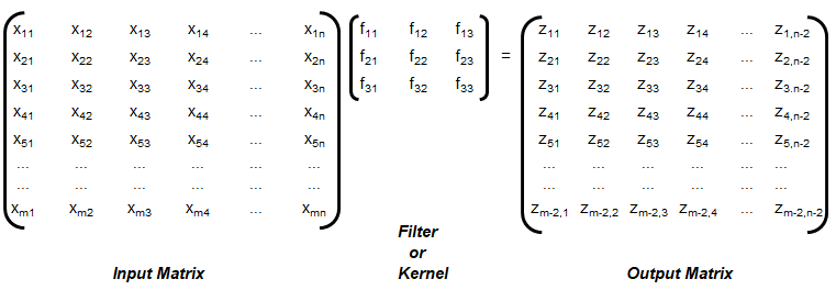
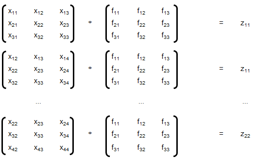
The convolution explained above is known as 'valid', without padding. Note that the size of output matrix has reduced by 2 in each dimension. Sometimes, padding is used where elements or layers of pixels are added all around, that is p rows and p columns are added to the input matrix with (conventionally) zeros. This helps get the output matrix of same size as that of input matrix. This is known as 'same' convolution. Similarly, the "strided convolution" use matrix multiplications in 'strides' or 'steps' where more than 1 rows and columns are stepped in the calculation of zij.
Convolution is a general method to create filter effect for images where a matrix is applied to an image matrix and a mathematical operation (generally) comprising of integers. The output after convolution is a new modified filtered image with a slight blur, Gaussian blur, edge detection... The smaller matrix of numbers or fractions that is used in image convolutions is called a Kernel. Though the size of a kernel can be arbitrary, a 3 × 3 is often used. Some examples of filters are:
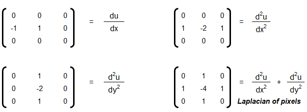
Following OCTAVE script produces 7 different type of images for a given coloured image as input.
The Sobel kernel may not be effective at all for images which do not have sharp edges. The GNU OCTAVE script used to generate these image enhancements and convolutions is described here.%In general Octave supports four different kinds of images % gray scale images|RGB images |binary images | indexed images % [M x N] matrix |[M x N x 3] array |[M x N] matrix | [M x N] matrix %class: double |double, uint8, uint16 |class: logical | class: integer %The actual meaning of the value of a pixel in a grayscale or RGB image depends %on the class of the matrix. If the matrix is of class double pixel intensities %are between 0 and 1, if it is of class uint8 intensities are between 0 and 255, %and if it is of class uint16 intensities are between 0 and 65535. %A binary image is an M-by-N matrix of class logical. A pixel in a binary image %is black if it is false and white if it is true. %An indexed image consists of an M-by-N matrix of integers and a Cx3 color map. %Each integer corresponds to an index in the color map and each row in color %map corresponds to an RGB color. Color map must be of class double with values %between 0 and 1.
The elements of a kernel must sum to 1 to preserve brightness: example of valid kernels are kernel_1 = np.array([ [-1, -1, -1], [-1, 9, -1], [-1, -1, -1] ]) ≡ kernel_2 = 1/9*np.array([ [1, 1, 1], [1, 1, 1], [1, 1, 1] ]). gauss_kernel = 1/16 * np.array([ [1, 2, 1], [2, 4, 2], [1, 2, 1] ]). Unweighted smoothing, weighted smoothing (Gaussian blur), Sharpening and Intense Sharpening Kernels respectively are described below
|1   1   1|      |0   1   0|      | 0   -1     0|     |-1   -1   -1|
|1   1   1|      |1   4   1|      |-1    5    -1|     |-1    9   -1|
|1   1   1|      |0   1   0|      | 0   -1     0|     |-1   -1   -1|
Laplacian Filter: Laplacian filter often refers to the simple 3 × 3 FIR (Finite Impulse Response) filter. The zero-crossing property of the Laplacian filter is used for edge location.
[ 0  −1   0
 −1   4  −1
  0  −1   0]
There are many other filters such as Sepia effect filter, Emboss effect, Mexican hat filter. filter_mex_hat = np.array([ [0, 0, -1, 0, 0], [0, -1, -2, -1, 0], [-1, -2, 16, -2, -1], [0, -1, -2, -1, 0], [0, 0, -1, 0, 0] ]) mexican_hat_img = cv2.filter2D(img, -1, filter_mex_hat). sepia_kernel = np.array([ [0.272, 0.534, 0.131], [0.349, 0.686, 0.168], [0.393, 0.769, 0.189] ]). sepia_img = cv2.transform(img, sepia_kernel).
Some standard colours and combination of RGB values are described below. These values can be easily studied and created using MS-Paint, edit colours option.
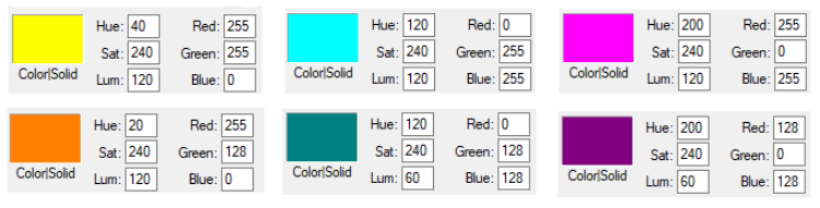
Pixels, DPI, PPI and Screen Resolution
As explained above, images are stored as pixels which are nothing but square boxes of size (in classical definition) 1/72 x 1/72 [in2] with colour intensity defined as RGB combination. However, the dimensions of a pixel are not fixed and is controlled by Pixels per Inch (PPI) of the device. Thus, size of pixel = physical size [inches] of the display / PPI of the display. Or PPI of a display device = 1/(Screen Size) x [(Horizontal Pixels)2 + (Vertical Pixels)2]0.5. Following pictures demonstrate the concept of pixels used in computer through an analogy of colour boxes used by the artist in MS-Excel.
![]()
![]()
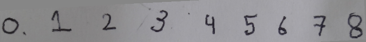
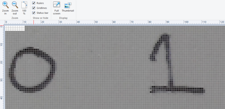
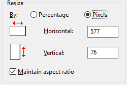
NumPy and SciPy arrays of image objects store information as (H, W, D) order (also designated as axis=0, axis=1 and axis=2 respectively. The values can be transposed as img = transpose(-1, 0, 1) = (D, W, H) = transpose(2, 0, 1). Here, (H, W, D) can be access either by (0, 1, 2) or (-3, -2, -1). The EGBA format of image adds alpha channel to describe opacity: α = 255 implies fully opaque image and α = 0 refers to fully transparent image. On a grayscale image, NumPy slicing operation img[:, 10:] = [0, 0] can be used to set 10 pixels on the right side of image to '0' or 'black'. img[:, :10] = [0, 0] sets 10 pixels on the left column to '0'.
The images when read in OCTAVE and pixel intensities converted into a text file results in following information. Note that the pixel intensity in text file is arranged by walking though the columns, that is the first 76 entries are pixels in first column in vertical direction.
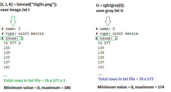
Even though the text file contains one pixel intensity per row, the variables I and G are matrices of size 76 x 577 x 3 and 76 x 577 respectively. The rows with entries "76 577 3" and "76 577" are used to identify the size of the matrices. The portion of image from row numbers from 100 to 250 and column numbers from 500 to 750 can be accessed as image_cropped = image[100:250, 500:750].
As explained earlier, type uint8 stands for unsigned (non-negative) integers of size 8 bit and hence intensities are between 0 and 255. The image can be read back from text file using commands: load("image.txt"); imshow(I); Note the text file generated by this method contains few empty lines at the end of the file and should not be deleted. The text file should have at least one empty line to indicate EOF else it will result in error and the image will not be read successfully.warning: imshow: only showing real part of complex image
warning: called from
imshow at line 177 column 5
Now, if the pixel intensities above 100 are changed to 255, it results in cleaned digits with sharp edges and white background. In OCTAVE, it is accomplished by statement x(x > 100) = 255. In Numpy, it is x[x > 100] = 255. You can also use & (and) and | (or) operator for more flexibility, e.g. for values between 50 and 100: OCTAVE: A((A > 50) & (A < 100)) = 255, Numpy: A[(A > 50) & (A < 100)] = 255. For a copy of original array: newA = np.where(A < 50, 0, A)
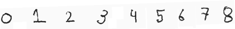
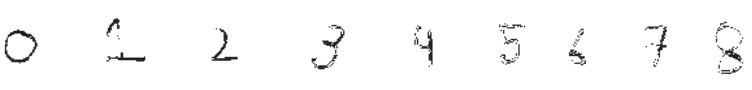
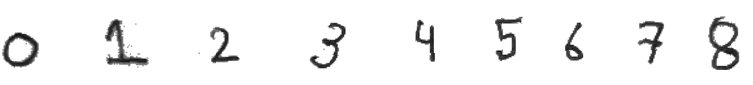
Attributes of Image Data
The images has two set of attributes: data stored in a file and how it is displayed on a device such as projectors. There are terms such as DPI (Dots per Inch), PPI (Pixels per Inch), Resolution, Brightness, Contrast, Gamma, Saturation... This PDF document summarizes the concept of DPI and image size. An explanation of the content presented in the PDF document can be viewed in this video file.
The video can be viewed here.Image File Types: PNG-8, PNG-24, JPG, GIF. PNG is a lossless format with option to have transparency (alpha channel). JPG files are lossy format and quality can be adjusted between 0 to 100%. JPG file cannot have transparency (alpha channel). PNG-8 or 8-bit version of PNG is similar to GIF format which can accommodate 256 colours and this format is suitable for graphics with few colours and solid areas having discrete-toned variation of colours. PNG-24 is equivalent to JPG and is suited for continuous-toned images with number of colours > 256. In effect, a JPG file shall have lesser size (disk space) than PNG with nearly equal or acceptable quality of the image. Screenshots should be saved as PNG format as it will reproduce the image pixel-by-pixel as it appeared originally on the screen.
This Python code uses Pillow to convert all PNG files in a folder into JPG format.
Image Filtering and Denoising
Image filtering is also known as Image Masking. The masking process is similar to a 'mask' or 'cover' we use for our body parts such as face. There are various types of noises that gets into scanned images or even images from digital camera. Gaussian, salt-and-pepper... are few of the names assigned to the type of noises. The concepts applicable to image enhancements are Edge Enhancement = Edge Sharpening, Convolution Filters, Remove Reflection, Glare and Shadow Removal, See-through corrections (visible text of underlying page), Despeckle, Smudge and Stains removal, JPEG compression artefacts, GIF compression pixelization and dot shading...CLAHE (Contrast Limited Adaptive Histogram Equalization) - worked well with for local contrast enhancement. Using different color space, such as HSV/Lab/Luv instead of RGB/BGR helps remove glares. The methods applicable to Document Imaging Applications (scanned texts) may not be effective to Photographic Image Applications (such as X-ray and Computer Tomography Scan images). Some of the requirements of denoising are removal of small noises, deletion of random or lonely pixels, thinning of characters of text in an image... The method to denoise or remove imperfections in an image is generally a two-step process: image segmentation followed by morphological operations.Denoising using skimage, OpenCV: This Python code uses Total Variance method to denoise an image. This method works well for random Gaussian noises but may not yield good result for salt and pepper noise.
| PIL | OpenCV |
| ImageFilter.BLUR | cv2.blur(src, kszie) |
| ImageFilter.MaxFilter(ksize) | cv2.dilate |
| ImageFilter.DETAIL | cv2.filter2D |
| ImageFilter.EDGE_ENHANCE | cv2.Sobel, cv2.Scharr, cv2.Laplacian, cv2.Canny |
| PIL.ImageFilter.EDGE_ENHANCE_MORE | |
| PIL.ImageFilter.EMBOSS | cv2.filter2D |
| PIL.ImageFilter.FIND_EDGES | cv2.Canny |
| PIL.ImageFilter.SMOOTH | cv2.GaussianBlur, cv2.MedianBlur, cv2.bilateralFilter |
| PIL.ImageFilter.SMOOTH_MORE | cv2.GaussianBlur, cv2.MedianBlur, cv2.bilateralFilter |
| PIL.ImageFilter.SHARPEN | cv2.filter2D |
| PIL.ImageFilter.GaussianBlur(radius) | cv2.GaussianBlur(src, ksize, sigmaX) |
This code uses Non-Local Mean (NLM) Algorithm to denoise an image. This method works well for random Gaussian noises but may not yield good result for salt and pepper noise.
OpenCV have algorithms termed as fastNlMeanDenoising with 4 variants: astNlMeansDenoising() - works with a single grayscale images, fastNlMeansDenoisingColored() - works with a color image, fastNlMeansDenoisingMulti() - works with image sequence such as videos (grayscale images), fastNlMeansDenoisingColoredMulti() - same as previous one but for color images. As per document, "Noise expected to be a Gaussian white noise." Gaussian white noise (GWN) is a stationary and ergodic random process with zero mean that is defined by fundamental property: "any two values of GWN are statistically independent no matter how close they are in time." Thus, these methods shall not work well on images containing texts such scanned copies of a textbook.Filter2D for removing speckles and isolated pixels: Blob is a group of connected pixels in an image that share some common property such as area, grayscale value, inertia, circularity...
kernel = np.ones((3,3), dtype=np.uint8)
kernel[1,1] = 0

# Create a sample (image) array that shows the 'blob' features
srcImg = np.array(
 [[1,0,1,1,1,0,0,0],
  [0,0,0,0,1,1,0,0],
  [1,0,1,1,1,1,1,1],
  [1,1,1,1,1,1,1,1],
  [0,0,1,1,1,0,1,1],
  [1,1,1,1,1,1,1,1],
  [1,1,1,0,1,1,0,1],
  [1,1,1,1,1,1,1,1]], dtype=np.uint8)

#input array needs to be converted to int8 or float32
srcImg = np.float32(srcImg)

mask = cv2.filter2D(srcImg, -1, kernel, borderType=cv2.BORDER_CONSTANT)
srcImg[np.logical_and(mask==8, srcImg==0)] = 1
cv2.imwrite('imgFiltered2D.png', srcImg*255)
| Input Image | Output Image |
 |  |
| 3 isolated pixels present | 3 isolated pixels removed |
cv2.filterSpeckles(bw_image_16bit, 'newVal' to paint-off the speckles, 'maxSpeckleSize' maximum number of pixels to be considered in a speckle, 'maxDiff' between neighbor disparity pixels to put them into the same blob) can be used to get similar output.
srcImg = cv2.filterSpeckles(srcImg, 1, 2, 100)[0]. img_blurred = cv2.blur(image, (5, 5)) where (5, 5) is the kernel size.This Python script uses Median Blur and Histogram Equalization to denoise a coloured image. Median Filters do not work well on texts as it filters out (or chip away) portions of characters. For median blur, kernel size should be an odd number else cv2 shall throw an error. Median filters work well on photographic images without text. Filters that are designed to work with gray-scale images shall not work with colour images. scikit-image provides the adapt_rgb decorator to apply filters on each channel of a coloured image.
Excerpt from scikit-image docs: "Removing small objects in grayscale images with a top hat filter: the top-hat transform is an operation that extracts small elements and details from given images. A white top-hat transform is defined as the difference between the input image and its (mathematical morphology) opening."
This is another code which uses Dilation, Blurring, Subtraction and Normalization to denoise an image and make the background white. This method applies well on scanned documents containing text and is compared with Adaptive Threshold option available in OpenCV. The adaptive threshold (such as OTSU thresholding) does not require a global threshold value and it can be further improved by splitting (tiling) the image into smaller rectangular segments for local background normalization (as explained in the page leptonica.org/binarization.html). OTSU method is an statistical method which minimizes in-class variance and maximizes between-the-class variance. Here, class refers to "set of pixels belong to a region". "Leptonica is a pedagogically-oriented open source library containing software that is broadly useful for image processing and image analysis applications."
Image Thresholding: This is a process of converting pixel value above or below a threshold to an specified value. This operation can be used to segment an image. For example, a grayscale image can be converted to black-and-white by converting all pixels having intensity value ≤ 64 to 0. Image thresholding is used to change the background of scanned text into white. One can manually calculate the histogram of dominant pixel intensities using cv2.CalcHist() or numpy.histogram or pyplot.hist() from matplotlib which can be further used to define threshold colour intensity value.
The grayscale images contain 256 shades of gray! That means if you have to convert the image into binary black and white, any intensity between 0 and 255 are noise! The thresholding produces jagged (stair-stepped) edges as a rule than exception. This is a common issue with threshold when if text is 'thin', the gaps in the letters appear after threshold. On the other hand when fonts are 'thick', the letters start merging (merged characters and character erosion).The approach to use dilution followed by erosion fuses neighboring texts in the dilution step which cannot be separated in the subsequent erosion step. Increasing the resolution of input image by scaling up and applying dilution followed by erosion are sometimes helpful but not much as the image has to be scaled down again.
def imageThreshold(imgName, thresh_global, blur_kernel, adapt_kernel):
  img = cv2.imread(imgName, cv2.IMREAD_GRAYSCALE)
  assert img is not None, "File could not be read, check with os.path.exists()"
  img_blurred = cv2.medianBlur(img, blur_kernel)
  methods = [cv2.THRESH_BINARY, cv2.ADAPTIVE_THRESH_MEAN_C,
    cv2.ADAPTIVE_THRESH_GAUSSIAN_C]
  ret, thresh_binary = cv2.threshold(img, thresh_global, 255, methods[0])
  thresh_adapt_mean = cv2.adaptiveThreshold(img, 255, methods[1],
    methods[0], adapt_kernel, 2)
  thresh_adapt_gauss = cv2.adaptiveThreshold(img, 255, methods[2],
    methods[0], adapt_kernel, 2)

  titles = ['Original Image', 'Global Thresholding',
    'Adaptive Mean Thresholding', 'Adaptive Gaussian Thresholding']
  images = [img, thresh_binary, thresh_adapt_mean, thresh_adapt_gauss]
  cv2.imwrite('Gauss_Threshold.png', thresh_adapt_gauss)
  return titles, images
Excerpt from scikit-image: "If the image background is relatively uniform, then you can use a global threshold value. However, if there is large variation in the background intensity, adaptive thresholding (or local or dynamic thresholding) may produce better results. Note that local is much slower than global thresholding. Otsu's threshold method can be applied locally. For each pixel, an optimal threshold is determined by maximizing the variance between two classes of pixels of the local neighborhood defined by a structuring element."
def plot_multiple_images(titles, images, n_rows, img_array=True):
  n = len(images)
  n_cols = math.ceil(n / n_rows)
  for i in range(n):
    if img_array:
      image_i = images[i]
    else:
      image_i = cv2.imread(images[i])
    plt.subplot(n_rows, n_cols, i+1), plt.imshow(image_i, 'gray')
    plt.title(titles[i], fontsize=9)
    plt.xticks([]), plt.yticks([])
  plt.show()
titles, images = imageThreshold('Input.png', 127, 3, 7)
plot_multiple_images(titles, images, 2, True)


for rad in range(1, 4):
  kernel = cv2.getStructuringElement(MORPH_ELLIPSE, Size(2*rad+1, 2*rad+1))
  morph = cv2.morphologyEx(morph, cv2.MORPH_CLOSE, kernel)
  morph = cv2.morphologyEx(morph, cv2.MORPH_OPEN, kernel)
Image Masking
The mask operation works on an input image and a mask image with logical operator such as AND, NAND, OR, XOR and NOT. An XOR (eXclusive OR) operation is true if and only if one of the two pixels is greater than zero, but both pixels cannot be > 0. The bitwise NOT function flips pixel values that is pixels that are > 0 are set to 0, and all pixels that are equal to 0 are set to 255. RGB = [255 255 255] refers to 'white' colour and RGB = [0 0 0] denotes a perfectly 'black' colour.
- AND: A bitwise AND is true (= 1 or 255) if and only if both pixels are > 0. In other words: white + anycolor = anycolor, black + anycolor = black.
- OR: A bitwise OR is true (=1 or 255) if either of the two pixels is > 0. With bitwise_or: white + anycolour = white, black + anycolour = anycolour.
- XOR: A bitwise XOR is true (=1 or 255) if and only if one of the two pixels is > 0, but not both are zero.
- NOT: A bitwise NOT inverts the on (1 or 255) and off (0) pixels in an image.
The list comprehension statement in NumPy can be used to convert image pixels based on threshold directly: img = [0 if img_pixel > thresh_intensity else img_pixel for img_pixel in img]. This is an IF condition inside a FOR loop and it needs to be read backward to understand the logic behind this one liner.
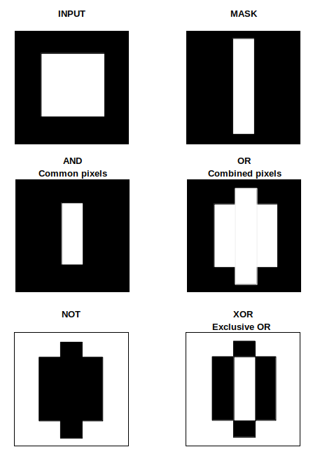
[expression for item in list if conditional]
for item in list:
  if conditional:
    expression

[expr_1 if condition_1 else expr_2 for item in list]
for item in list:
  if condition_1:
    expr_1
  else:
    expr_2
Distance Masking: Determine the distance of each pixel to the nearest '0' pixel that is the black pixel. cv2.add(img1, img2) is equivalent to numPy res = img1 + img2. There is a difference between OpenCV addition and Numpy addition. OpenCV addition is a saturated operation while Numpy addition is a modulo operation. cv2.add(250, 25) = min(255, 275) = 255, np.add(250, 25) = mod(275, 255) = 20. Note there is no np.add function, used for demonstration purposes only.
| Input Image | Mask Image | Operation | Outcome of Operation |
| Binary or Grayscale | Binary | OR | Pixels having value 0 in mask set to 0 in output, other pixels from input image retained |
| Input Image | Mask Image | AND | Pixels having value 0 in mask set to 1 or 255 in output, other pixels from input image retained |
Circular Crop: This Python code uses OpenCV to create a circular crop of an image. The input image and cropped image are shown below. In HTML, border-radius property can be set to 50% to make the image cropped to a circle.

Alternatively, the image can be read into a NumPy array and pixels beyond each channel beyond the disk can be set to desired colour. This Python code uses OpenCV and NumPy array to create a circular crop of an image. The image is read using OpenCV, the BGR channels are extracted as NumPy arrays and then the pixels of each channel are set to white beyond the boundary of circular disk. Finally, BGR channels are merged to create the coloured image. Following image describes the formula required to add a round to the corners of an image

def createRoundedCorners(image, radius):
  img = cv2.imread(image)
  img_w, img_h = img.shape[1]-1, img.shape[0]-1
  for w in range(0, radius):
    ht = radius - int(np.sqrt(2*radius*w - w * w))
    for h in range(0, ht):
      img[h, w] = 255
      img[h, img_w - w] = 255
      img[img_h - h, w] = 255
      img[img_h - h, img_w - w] = 255
  return img
Unsharp Mask
Unsharp mark is a bit misnomer as it is used to sharpen an image. Unsharp mask is equivalent to blurred version of image where sharpened image = original image - blurred image. Unsharp mask locates pixels that differ from neighbouring pixels by the specified threshold (delta). It then increases the contrast of the pixels by the amount specified. For pixels within the specified radius, the lighter (or brighter) pixels get lighter (or brighter), the dark ones get darker.Excerpt from scikit-image docs: "Unsharp masking is a linear image processing technique which sharpens the image. The sharp details are identified as a difference between the original image and its blurred version. These details are then scaled, and added back to the original image: enhanced image = original + amount * (original - blurred). The blurring step could use any image filter method, e.g. median filter, but traditionally a Gaussian filter is used. The radius parameter in the unsharp masking filter refers to the sigma parameter of the Gaussian filter."
Connected Component Labeling
This Python script can be used to update an image background to white. This code uses Connected Component Labeling (CCL) method to remove the dark patches. The code customised for all images inside a folder can be found here. In case the text contains shadow in the background, the gray-scale image, the contrast has to be adjusted to accentuate the dark grays from the lighter grays - this can be achieved by imgGray = cv2.multiply(imgGray, 1.5) though the multiplier 1.5 used here needs to be worked out by trial-and-error. 1.1 is a recommended start value. Gaussian Blur and morphological operations such as erosion and dilation would be required to make the text sharper: kernel = np.ones((2, 1), np.uint8), img = cv2.erode(img, kernel, iterations=1). "Using Machine Learning to Denoise Images for Better OCR Accuracy" from pyimagesearch.com is a great article to exploit the power of ML to denoise images containing dominantly texts and noises. Before applying CCL, the image has to be converted into a binary format: threshImg = cv2.threshold(grayImg, 0, 255, cv2.THRESH_BINARY_INV | cv2.THRESH_OTSU)[1] can be used for this. cv2.THRESH_BINARY_INV applies threshold and inverts image colour to black background and white foreground.
nLables, labels, stats, centroids = cv2.connectedComponentsWithStats( imgBlackBackground, 8, cv2.CV_32S ) or outputCCWS = cv2.connectedComponentsWithStats(...) and (nLables, labels, stats, centroids) = outputCCWS, 8 is connectivity type (another option is 4), CV_32S is output image label type
- nLabels = total number of unique labels. The background is label 0, and the additional objects are numbered from 1 to nLabels-1.
- labels = list of masks created from connected components (CC) - spatial dimensions same as input image
- stats = statistical information of CC: cv2.CC_STAT_LEFT = stats[:, 0], cv2.CC_STAT_TOP = stats[:, 10], cv2.CC_STAT_WIDTH = stats[:, 2], cv2.CC_STAT_HEIGHT = stats[:, 3], cv2.CC_STAT_AREA = stats[:, 0] = stats[:, 4]
- Get maximum area of CC: max(stats[1:, -1]). Array of areas of connected components can be created using outputCCWS[2][:, 4].
- Get CC with 3 highest areas: sorted(stats[1:, -1], reverse=True)[:3]
- Get second highest area of CC: max( stats[1:, -1].remove(max(stats[1:, -1])) ) - note that this is a destructive approach and the items from list get deleted.
- Save ith CC label: cclMask = (labels == i).astype("uint8") * 255, cv2.imwrite( "ccComp_i.png", cv2.bitwise_or( cclMask)). Bitwise OR operation is needed to invert background colour to white - note that cv2.THRESH_BINARY_INV was used during threshold operation.
- Further dilation and/or erosion operation may need to be performed on each of the Connected Components to remove isolated pixels, tiny holes and irregular shapes.
contours_sorted = sorted(contours, key = cv2.contourArea, reverse = True)
for c in contours_sorted[1:-1]:
  x, y, w, h = cv2.boundingRect(c)
  input_img[y:y+h, x:x+w] = 255
cv2.imwrite('imgDespecled.png', input_img)

ImageMagick has options to use Connected Component Labelling technique to remove noises such as random pixels and despeckle an image. Excerpts from webpage: "Connected-component labelling (alternatively connected-component analysis, blob extraction, region labelling, blob discovery, or region extraction) uniquely labels connected components in an image. The labelling process scans the image, pixel-by-pixel from top-left to bottom-right, in order to identify connected pixel regions, i.e. regions of adjacent pixels which share the same set of intensity values."
Find background colour of an image: there is no unique and universal method to find the background colour of an image. One direct approach is to get the pixel value with the highest occurrence. This may not yield correct value if two pixels are nearly equal. Depending upon type of image, the method can be adjusted. For example, an image containing (lot of) texts only, the method to find pixel value of highest occurrence may give correct value of background color. Alternatively, in such images when there are no or sparse noises present, finding the pixel of maximum continuous occurrence in each row or column shall yield (universally) correct background colour.
Image Denoising using ML: Noise2Void is a widely used denoising algorithm, and is readily available from the n2v python package which isbased on TensorFlow. Refer: github.com/CAREamics/careamics - "CAREamics is a PyTorch library aimed at simplifying the use of Noise2Void and its many variants and cousins (CARE, Noise2Noise, N2V2, P(P)N2V, HDN, muSplit)." Articles describing the underlying principles are [1]"Noise2Noise: Learning Image Restoration without Clean Data" by Jaakko Lehtinen et al. [2]"Noise2Void - Learning Denoising from Single Noisy Images" by Alexander Krull et al. [3]"Noise2Self: Blind Denoising by Self-Supervision" by Joshua Batson and Loic Royer.
Pixel Multiplication
Also known as Graylevel scaling (and not same as geometrical scaling), this operation can be used to brighten (scaling factor > 1) or darken (scaling factor < 1) an image. If the calculate value of pixel after multiplication is > maximum allowed value, it is either truncated to the maximum value or wrapped-around the minimum allowed pixel value. For example, a pixel value of '200' when scaled by a factor 1.3, the new value of 260 shall get truncated to 255 or wrapped to 5 (= 260 - 255).There is similar operation "Image Segmentation with Distance Transform and Watershed Algorithm" available at docs.opencv.org/3.4/d2/dbd/tutorial_distance_transform.html. Here, OpenCV function distanceTranform is used to obtain derived representation of a binary image, where the value of each pixel is replaced by its distance to the nearest background pixel.
Adapted from stackoverflow.com/../what-processing-steps-should-i-use-to-clean-photos-of-line-drawings, the Python + OpenCV code attached here can be used to clean image as shown below.
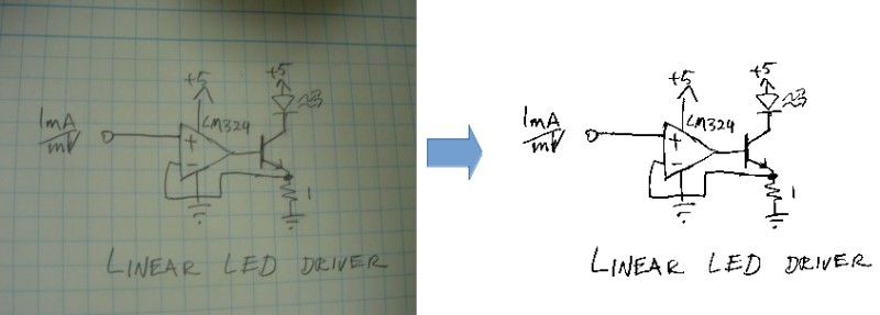
Morphological Operations
Morphology refers to "the study of the forms / shape / structure of things". In linguistics, it is study about pattern of word formation (inflection, derivation, and compounding). Image processing methods that transform images based on shapes are called Morphological Transformations. Erosion is the morphological operation that is performed to reduce the size of the foreground object. Dilaton is opposite of erosion. Thus, thickness of fonts can be reduced using erosion and vice versa. Bright regions in an image tend to “get brighter” after Dilation, which usually results in an enhanced image. Removing noise from images is one of the application of morphological transformations. Morphological operators require Binary Images which are images whose pixels have only two possible intensity values. They are normally displayed as black and white and the two values are 0 for black, and either 1 or 255 for white.
Erosion is also known as minimum filter which replaces or removes objects smaller than the structure (thinning operation - removes foreground pixels). Similarly, dilation is called maximum filter (thickening operation - adds foreground pixels). A structuring element or kernel is a simple shape used to modify an image according to the shape locally fits or misses the image. A structuring element is positioned all possible locations in the image and thus sometime may not fit on boundary pixels. Note that morphological operations such as Erosion and Dilation are based on set operations whereas convolutions are based on arithmetic operations.
Tutorial at docs.opencv.org titled "Extract horizontal and vertical lines by using morphological operations" demonstrates how horizontal lines can be removed as shown below.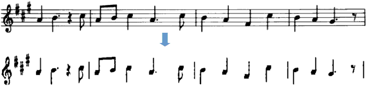
Excerpt from docs.opencv.org: "During erosion a pixel in the original image (either 1 or 0) will be considered 1 only if all the pixels under the kernel is 1, otherwise it is eroded (made to zero)." Excerpt from pyimagesearch.com: "A foreground pixel in the input image will be kept only if all pixels inside the structuring element are > 0. Otherwise, the pixels are set to 0 (i.e. background)." From OpenCV tutorial: "The kernel B has a defined anchor point, usually being the center of the kernel. As the kernel B is scanned over the image, we compute the maximal pixel value overlapped by B and replace the image pixel in the anchor point position with that maximal value. As you can deduce, this maximizing operation causes bright regions within an image to "grow" (therefore the name dilation)."
As you may have realized, none of the 3 definitions quoted above is clear where the use of 0 and 1 for boolean and pixel intensities are mixed-up. Let's see the effect of kernel and erosion with following examples.
| erosion = cv2.erode(img, np.ones((3, 3), np.uint8), iterations = 1) | ||
| Image with black background | Image after erosion | Image after Dilation |
 |  |  |
| Image with white background | Image after erosion | Image after Dilation |
 |  |  |
| As evident now, erosion adds black pixels and depending upon the background colour, the thickening (white background) or thinning (black background) effect can be observed. | ||
A key consideration while using morphological operations is the background colour of the image. Should it be white or black? Is the kernel definition dependent on whether background of image is white or black? docs.opencv.org recommends: "(Always try to keep foreground in white)". If you have an image with white background, in order to comply this recommendation, use whiteForeground = cv2.bitwise_not( blackForeground ) before erosion and then blackForeground = cv2.bitwise_not( whiteForeground ) after erosion. This short piece of code describes these steps.
A = Image, B = Kernel --- Erosion = A ⊖ B, Dilation: A ⊕ B, Opening: A o B = (A ⊖ B) ⊕ B, Closing: A ⊚ B = (A ⊕ B) ⊖ B. A combination of morphological operations can be used for smoothing and dirt removal. For example: convert image background to black -> dilate to remove white dots (lonely pixels in original image) -> erode to bring text to original thickness -> invert background colour of image back to white. The operations can be chain-combined as: k_blur = ((3, 3), 1), k_erode = (5, 5), k_dilate = (3, 3). cv2.imwrite( 'imgMorphed.png', cv2.dilate( cv2.erode( cv2.GaussianBlur( cv2.imread('Input.png', 0) / 255, k_blur[0], k_blur[1]), np.ones(k_erode)), np.ones(k_dilate) ) * 255 ).
cv2.getStructuringElement(cv2.MORPH_RECT, (50,1)): this can be used to create a horizontal line to remove such lines from an image. cv2.MORPH_RECT, (1, 50) can be used to create a vertical line.
Rectangular Kernel: cv2.getStructuringElement(cv2.MORPH_RECT,(3,3))
array([[1, 1, 1],
       [1, 1, 1],
       [1, 1, 1]], dtype=uint8)

Elliptical Kernel: cv2.getStructuringElement(cv2.MORPH_ELLIPSE,(5,5))
array([[0, 0, 1, 0, 0],
       [1, 1, 1, 1, 1],
       [1, 1, 1, 1, 1],
       [1, 1, 1, 1, 1],
       [0, 0, 1, 0, 0]], dtype=uint8)

Cross-shaped Kernel: cv2.getStructuringElement(cv2.MORPH_CROSS,(3,3))
array([[0, 1, 0],
       [1, 1, 1],
       [0, 1, 0], dtype=uint8)
Main Function
import cv2, sys
import numpy as np
def imgMorphOperation(imgName, kernel_size, imgType='File', morph='Opening'):
  #imgType = 'File'  or NumPy 'Array' if already loaded by cv2.imread
  #morph = 'Opening', 'Closing', 'Dilation', 'Erosion'
  if imgType == 'File':
    img = cv2.imread(imgName, cv2.IMREAD_GRAYSCALE)
  else:
    img = imgName
  # Otsu's thresholding
  ret,img = cv2.threshold(img, 0, 255, cv2.THRESH_BINARY+cv2.THRESH_OTSU)

  kernel = np.ones((kernel_size, kernel_size), np.uint8)
  if morph == 'Opening':
    imgMorphed = cv2.morphologyEx(img, cv2.MORPH_OPEN, kernel)
  elif morph == 'Erosion':
    imgMorphed = cv2.erode(img, kernel, iterations = 1)
  elif morph == 'Dilation':
    imgMorphed = cv2.dilate(img, kernel, iterations = 1)
  elif morph == 'Closing':
    imgMorphed = cv2.morphologyEx(img, cv2.MORPH_CLOSE, kernel)
  else:
    print("\nMorphological operation not defined! Exiting. \n")
    sys.exit()

  return imgMorphed
Original Image: Reference: "Morphological Image Processing" by Preechaya Srisombut, Graduate School of Information Sciences and Engineering,Tokyo Institute of Technology
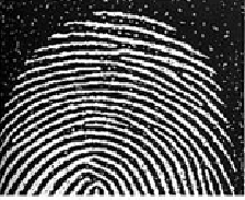
imgName = 'fingerPrintWithNoise.png'
imgEroded = imgMorphOperation(imgName, 3, imgType='File', morph='Erosion')
cv2.imwrite('fingerPrintEroded.png', imgEroded)
Image after First Erosion
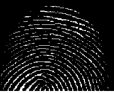
imgDilated1 = imgMorphOperation(imgEroded, 3, imgType='Array', morph='Dilation')
cv2.imwrite('fingerPrintDilate1.png', imgDilated1)
Image after First Dilation
imgDilated2 = imgMorphOperation(imgDilated1, 3, imgType='Array', morph='Dilation')
cv2.imwrite('fingerPrintDilate2.png', imgDilated2)
Image after Second Dilation
imgFinal = imgMorphOperation(imgDilated2, 3, imgType='Array', morph='Erosion')
cv2.imwrite('fingerPrintDenoised.png', imgFinal)
Denoised Image after Second Erosion
Image deskewing
First thing first: to deskew an image, remove the noise especially around the boundary or edges of the image else the contour of largest area shall be the one formed by continuous dark patches at the edges (almost the size of the image itself). This is the method of straightening a rotated image - a mandatory step in image pre-processing before feeding the cleaned-up image to an Optical Character Recognition (OCR) tool. The recommended steps are described below:- Convert the image to gray scale
- Apply slight blurring to decrease intensity of noise in the image
- Invert and maximize the colors of image by thresholding to make text block detection easier, thus making the text white and changing background to black
- Merge all printed characters of the block via dilation (expansion of white pixels) to find text blocks
- Use larger kernel on X axis to get rid of all spaces between words and a smaller kernel on Y axis to blend in lines of one block between each other, but keep larger spaces between text blocks intact
- Find areas of the text blocks of the image
- Use simple contour detection with minimum area rectangle for all the block of text
- Determine skew angle: angle the texts need to be rotated to make them aligned to page: there are various approaches to determine skew angle, such as average angle of all text blocks, angle of the middle block or average angle of the largest, smallest and middle blocks. Simple one using the largest text block works fine in most of the cases.
import cv2
import numpy as np
def cleanTextImage(img, min_area: int):
  '''
  Ref: stackoverflow.com/ ... /clean-text-images-with-opencv-for-ocr-reading
  This code requires (assumes) properly binarized white-on-black image (e.g.
  after grayscale conversion, black hat morphing and Otsu's thesholding).
  '''
  num_comps, labeled_pix, comp_stats, comp_centroids = \
    cv2.connectedComponentsWithStats(img, connectivity=4)

  # Get indices/labels of the remaining components based on the area stat
  # (skip the background component at index 0)
  comp_labels = [i for i in range(1,num_comps) if comp_stats[i][4] >= min_area]

  # Filter the labeled pixels based on the remaining labels,
  # assign pixel intensity to 255 (uint8) for the remaining pixels
  cln_img = np.where(np.isin(labeled_pix,comp_labels)==True,255,0).astype('uint8')

  return cln_img
Usage:
_,img = cv2.threshold(cv2.imread('In.jpg',0), 0,255,cv2.THRESH_BINARY+cv2.THRESH_OTSU)
cv2.imwrite('cln_img.jpg', cleanTextImage(img, 10))Template Matching
Similar to erosion and other morphological operations, there is another utility named Template Matching where an image template slides (similar to kernel or structuring elements - moving the patch one pixel at a time: left to right, up to down) and compares the template and overlapping patch of input image. At each location, a metric is calculated so it represents how "good" or "bad" the match at that location is (or how similar the patch is to that particular area of the source image). It returns a grayscale image, where each pixel denotes how much does the neighbourhood of that pixel match with template. The brighter pixels representing good match will have a value closer to 1, whereas a relatively darker pixel representing not so good match will have a value close to 0. If input image has the size (W x H) and template image is of size (w x h), output image will have a size of (W-w+1, H-h+1).The value of match and location of match from the metric calculated by cv2.matchTemplate() can be retried by min_val, max_val, min_loc, max_loc = cv2.minMaxLoc(result) to get the minimum and maximum value of 'match' as well the coordinates indicating the "top-left, bottom-right" corners for the bounding box. min_loc and max_loc are touples of (x, y).
import cv2 as cv
import numpy as np

img_rgb  = cv.imread('NoisyImage.png')
img_gray = cv.cvtColor(img_rgb, cv.COLOR_BGR2GRAY)

imgTemplate = np.array([[1, 1, 1, 1], [1, 0, 0, 1],
                        [1, 0, 0, 1], [1, 1, 1, 1]], np.uint8) * 255
w, h = imgTemplate.shape[::-1]
res = cv.matchTemplate(img_gray, imgTemplate, cv.TM_CCOEFF_NORMED)

# If multiple occurrences of match found, cv.minMaxLoc() won't give all
# the locations. In that case, thresholding needs to be used.
threshold = 0.8
loc = np.where(res >= threshold)
for pt in zip(*loc[::-1]):s
  #Add rectangle with red lines around matched patches
  #cv.rectangle(img_rgb, pt, (pt[0] + w, pt[1] + h), (0,0,255), 1)

  # Change pixels in the matched patches to white (255)
  img_gray[pt[1]:pt[1] + h, pt[0]:pt[0] + w] = 255
cv.imwrite('imageMatched.png', img_gray)
If np.uint8 is ignored in imgTemplate array definition, following error occurs in statement: res = cv.matchTemplate(img_gray, imgTemplate, cv.TM_CCOEFF). "cv2.error: OpenCV(4.7.0) /io/ opencv/ modules/ imgproc/ src/ templmatch.cpp: 1164: error: (-215: Assertion failed) (depth == CV_8U || depth == CV_32F) && type == _templ.type() && _img.dims() <= 2 in function 'matchTemplate'"
Find Contours
From docs.opencv.org/ ... /tutorial_py_contours_begin.html: Contours are curves joining all the continuous points (along the boundary), having same color or intensity. The contours are a useful tool for shape analysis and object detection and recognition. In OpenCV, finding contours is like finding white object from black background. So object to be found should be white and background should be black.
cv2.findContours() function is used to detect objects in an image. Usage: imgCont, contours, hierarchy = cv.findContours(threshold, cv.RETR_TREE, cv.CHAIN_APPROX_SIMPLE) where imgCont is modified image returned from findContour operation, contours is a Python list of all the contours in the image (each contour as a Numpy array of (x,y) coordinates of boundary points of the object). It accepts argument to specify Contour Retrieval Mode and Contour Approximation Method. This is especially useful to identify nested contours (object inside another object).cv2.RETR_LIST: It simply retrieves all the contours, but doesn't create any parent-child relationship thus they all belongs to same hierarchy level. cv2.RETR_TREE: It retrieves all the contours and creates a full family hierarchy list. cv2.RETR_CCOMP: This flag retrieves all the contours and arranges them to a 2-level hierarchy. Thus, external contours of the object (i.e. its boundary) are placed in hierarchy-1 and the contours of holes inside object (if present) is placed in hierarchy-2. cv2.RETR_EXTERNAL: If you use this flag, it returns only extreme outer flags. All child contours are left behind.
cv2.CHAIN_APPROX_SIMPLE removes all redundant points and compresses the contour for example for straight lines only end points are needed. cv2.CHAIN_APPROX_NONE stores all boundary points.
Draw Contours
cv.drawContours(img, contours, -1, (255, 255, 0), 2): cv2.drawContours function is used to draw any shape for which the boundary points are known. Its first argument is source image, second argument is the contours which should be passed as a Python list, third argument is index of contours (useful when drawing individual contour, -1 can be used to draw all contours), next argument is color and the last argument is thickness of boundary lines.Following function can be used to remove all horizontal lines from an image. Vertical lines can be removed by changing (kernel_size, 1) to (1, kernel_size).
def imgRemoveHorizLines(imgName, imgType='File', kernel_size=50):
  if imgType == 'File':
    image = cv2.imread(imgName)
  else:
    image = imgName
  imGray = cv2.cvtColor(image, cv2.COLOR_BGR2GRAY)
  thresh = cv2.threshold(imGray, 0,255, cv2.THRESH_BINARY_INV + cv2.THRESH_OTSU)[1]

  hr_krnl = cv2.getStructuringElement(cv2.MORPH_RECT, (kernel_size, 1))
  rm_hr = cv2.morphologyEx(thresh, cv2.MORPH_OPEN, hr_krnl, iterations=2)
  cnts = cv2.findContours(rm_hr, cv2.RETR_EXTERNAL, cv2.CHAIN_APPROX_SIMPLE)
  if len(cnts) == 2:
    cnts = cnts[0]
  else:
    cnts = cnts[1]

  for c in cnts:
    cv2.drawContours(image, [c], -1, (255,255,255), 3)
  cv2.imwrite('imgHorizLinesRemoved.png', image)
  return image
RUN LENGTH SMOOTHING ALGORITHM (RLSA): block segmentation and text discrimination method used in Document Image Processing to extract the region of interest (ROI) such as block-of-text, title, and content. This method can be used to remove text in images where content from next / previous page gets added while scanning pages from the books.
Animations using Python
Convert PNG to Animated GIF: Click here to get a Python script to convert a set of PNG file to animated GIF.
There are few requirements to be kept in mind while using VideoWriter in OpenCV else video writing fails silently - no valid video file is written: [1] All frames should of same size including number of channels [2] All images should be either coloured or black-and-white [3] If input images are monochrome (black and white or grayscale) type, it should be indicated with argument isColor = False or '0' such as cv2.VideoWriter('output.avi', fourcc, 25, size, 0) [4] The images must be in BGR format (and not RGB) or it will not write any video [5] FFmpeg should be configured properly [6] Try different codecs and see which one works or use "-1" in place of the codec flag and select one from the list [7] frameSize required by cv2.VideoWriter is (width, height) and not (height, width) which is the shape of image array resulting from cv2.imread or Image.open [8] Specify frames per second or FPS argument as type float [9] If folder or path does not exist, VideoWriter will fail silently.Animation of a sine wave. The Python code can be found here.
def rotateImageInCircle(images, icon_w, icon_h, radius):
  num_images = len(images)
  frame_w = ((icon_w + 2 * radius) // 2) * 2
  frame_h = ((icon_h + 2 * radius) // 2) * 2
  xc = frame_w // 2
  yc = frame_h // 2
  img_frames = []
  for theta in range(360):
    frame = np.ones((frame_h, frame_w, 3), dtype=np.uint8)*255
    for i, image in enumerate(images):
      img = cv2.resize(cv2.imread(image), (icon_h, icon_w))

      angle = (i/num_images + theta/360) * 2 * np.pi
      x = int(xc + radius * np.cos(angle))
      y = int(yc + radius * np.sin(angle))
      img_x = x - icon_w // 2
      img_y = y - icon_h // 2
      img_x = max(0, min(img_x, frame_w - icon_w))
      img_y = max(0, min(img_y, frame_h - icon_h))

      frame[img_y:img_y + icon_h, img_x:img_x + icon_w] = img
    img_frames.append(frame)
return frame_w, frame_h, img_framesImage to PDF
This Python code converts all the images stored in a folder into a PDF file.
Coordinate Transformation Matrices
If {X} is a row vector representing a 2D or 3D coordinates of a point or pixel, {X'} = [T] {X} where [T] is the transformation matrix. Thus: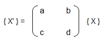
| Operation | a | b | c | d | Remark |
| Scaling | ≠ 0, ≠ 1 | 0 | 0 | ≠ 0, ≠ 1 | |
| Reflection about y-axis | -1 | 0 | 0 | 1 | |
| Reflection about x-axis | 1 | 0 | 0 | -1 | |
| Reflection about origin | < 0 | 0 | 0 | < 0 | |
| Shear | 0 | ≠ 0, ≠ 1 | ≠ 0, ≠ 1 | 0 | |
| Rotation: 90°CCW about origin | 0 | 1 | -1 | 0 | |
| Rotation: 180°CCW about origin | -1 | 0 | 0 | -1 | |
| Rotation: 270°CCW about origin | 0 | -1 | -1 | 0 | |
| Rotation: θ CCW about origin | cosθ | sinθ | -sinθ | cosθ | |
| Reflection about x-axis | -1 | 0 | 0 | 1 | |
| Reflection about x-axis | 1 | 0 | 0 | -1 | |
| Reflection about y = x | 0 | 1 | 1 | 0 | |
| Reflection about y = -x | 0 | -1 | -1 | 0 |
Rotation is assumed to be positive in right hand sense or the clockwise as one looks outward from the origin in the direction along the rotation axis. The right hand rule of rotation is also expressed as: align the thumb of the right hand with the positive direction of the rotation axis. The natural curl of the fingers gives the positive rotation direction. Note the the x-coordinate of the position vector will not change if rotation takes place about x-axis, y-coordinate of the position vector will not change if rotation takes place about y-axis and so on.
Scaling: if a = d and b = c = 0, uniform scaling occurs. A non-uniform expansion or compression will result if a = d > 1 or a = d < 1 respectively. Scaling looks like an apparent translation because the position vectors (line connecting the points with origin) are scaled and not the points. However, if the centroid of the image or geometry is at the origin, a pure scaling without apparent translation can be obtained.
Homogeneous coordinates: in the transformation matrices described in the table above, the origin of the coordinate system is invariant with respect to all of the transformation operations. The concept of homogenous coordinate system is used to obtain transformations about an arbitrary point. The homogenous coordinates of a non-homogeneous position vector {X Y} are {X' Y' h} where X = X'/h and Y = Y'/h and h is any real number. Usually, h = 1 is used for convenience though there is no unique representation of a homogenous coordinate system. Thus, point (3, 5) can be represented as {6 10 2} or {9 15 3} or {30 50 10}. Thus, a general transformation matrix looks like shown below. Note that every point in a two-dimensional plane including origin can be transformation (rotated, reflected, scaled...).
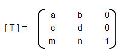
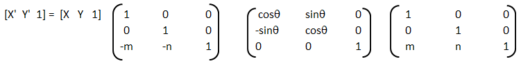
[T] = [T'] [R] [R'] [R]-1 [T']-1
Thus, the steps are:- Translate the line and the object both so that the line passes through the origin: the matrix [T'] in above concatenated matrix [T]
- Rotate the line and the object about the origin so that the line coincides with one of the coordiante axis: the matrix [R]
- Reflect the object about the line - the coordinate axis it coincides with: the matrix [R']
- Apply the inverse rotation above the origin using: the matrix [R]-1
- Apply the inverse translation to the original location: the matrix [T]-1
3D Transformations
The three-dimensional representation and display of an object is necessary for the understanding of the shape of the object. Additionally, the ability to translate (pan), rotate (dolly), scale (zoom), reflect and project help understand the shape of the object. Analogous to homogeneous coordinate system in 2D, a point in 3D space {X Y Z} can be represented by a 4D position vector {X' Y' Z' h} = {X Y Z 1} [T] where [T] is the transformation matrix similar to the one used in 2D case. A generalized 4 × 4 transformation matrix for 3D homogeneous coordinates is: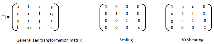
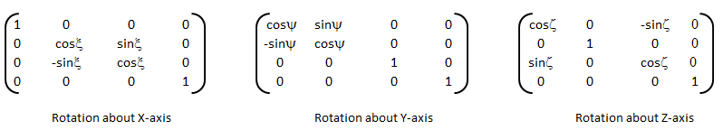
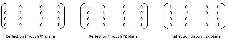

- Alpha Mask / Wipe Transition: Uses a grayscale mask image to gradually wipe / transition between 2 images. Alpha = Transparency
- Bars: Add colored bars around your video
- Blur/Sharpen: Adjust the blur/sharpness of the frame’s image - ffmpeg -i in.mp4 -vf "unsharp= luma_msize_x=7: luma_msize_y=7: luma_amount=2.5: enable= 'between(t, 2, 3)'" -y out.mp4
- Adjust the brightness and contrast of the frame’s image: A value of -1 for brightness makes the image black and value of +1 makes it white. Intermediate values can be used to adjust brightness. The value of contrast varies between -128 to +128 in OpenShot and controls sharpness or intensity or depth of the colour.
- Caption: Add text captions on top of your video - background alpha, padding, corner radius, font alpha, font size, text location... are some of the options available in OpenShot
- Chroma Key (Greenscreen): Replaces the color (or chroma) of the frame with transparency (i.e. keys out the color). This can be used to remove background colours in screen recording with web-cam such as OBS Studio. However, the background colour should be of any single uniform colour and not the green colour only.
- Color Saturation: Adjust the color saturation, 0 means black-and-white image and higher value increase the intensity of the colours
- Color Shift: Shift the colors of an image up, down, left, and right (with infinite wrapping)
- Crop: Crop out any part of your video
- Deinterlace: Remove interlacing from a video (i.e. even or odd horizontal lines)
- Hue: Adjust the hue / color of the frame’s image - this is used to create Colour Change Effect
- Negative: Negates the colors, producing a negative of the image - OpenShot does not provide any control on the attributes of the negative colors of the image
- Object Detector: Detect objects through the video
- Pixelate: Pixelate (increase or decrease) the size of visible pixels that is the effect reduces PPI of the image and hence it blurs the image
- Shift the image up, down, left, and right (with infinite wrapping) - this option separates and shows the 3 colour channels by horizontal and/or vertical shift specified - also known as Glitch Effect sometimes
- Stabilizer: Stabilize video clip to remove undesired shaking and jitter
- Wave: Distort the frame’s image into a wave pattern
Similarly, transition as the name suggests, indicates the method or style to switch between one clip (or frame) to another, such as to gradually fade (or wipe) between two clips. Thus, the most common location of a 'transition' is either at the start or end of the clip or image or keyframe. Direction of transitions adjust the alpha or transparency of the clip below it, and can either fade from opaque (dark) to transparent (default), or transparent to opaque. One interesting animation shown below is 'Cube' transition in PowerPoint and LibreOffice Impress which ensures continuity of information.
Following Python code generate frames to create Cube transition.
def frames_cube_transition(img1, img2, img_w, img_h, steps=50):
  transition_frames = []
  for i in range(steps):
    alpha = i / steps
    angle = alpha * np.pi/2
    m1 = np.float32([[1, 0, -img_w*   np.sin(angle)],  [0, 1, 0]])
    m2 = np.float32([[1, 0,  img_w*(1-np.sin(angle))], [0, 1, 0]])
    frame1 = cv2.warpAffine(img1, m1, (img_w, img_h))
    frame2 = cv2.warpAffine(img2, m2, (img_w, img_h))

    combined_frame = np.maximum(frame1, frame2)
    transition_frames.append(combined_frame)
  return transition_frames
Most of the open source program are better at dealing with images. However, the flexibility to deal with text are less and sometimes limited options are there. For example, to add scrolling credits a long text object is moved vertically to make it appear to be scrolling: appearing from the bottom and disappearing through the top. Blender version 3.6.1 does not have this as standard feature. An indirect way to do this is to create the image of the text and animate it bottom to top.
Animation: the visual appearance of a video and animations are same and hence a video is an animation and an animation is a video - to human eyes. Thus, the option to animate in a Video Editing program may be confusing initially. The feature 'animation' refers to ability to change few keyframes in the clip or the video such as zoom, pan or slide.
Example demonstration: Create a Zoom and Pan animation in OpenShot
- Step-1: Move the timeline where you want to begin to zoom
- Step-2: Right click on your clip, and choose Transform: this will display some interactive handles over the video preview
- Step-3: Drag the corner (while holding CTRL) to scale the image larger or smaller
- Step-4: Alternatively, use the Clip's properties to change the scale_x and scale_y, and location_x, and location_y properties
- Step-5: Drag the center circle handle to move the image
- Step-6: Move to the next position in the video, and repeat these steps.
Note that most of the 'rotation' codes are meant to rotate an images about z-axis which the axis perpendicular to the plane of computer screen. Rotation about x- and y-axis which are coplanar to computer screens requires homographic transformation which is a projective transformation between two planes. One example is available at answers.opencv.org/ ... /direct-formula-for-3d-rotation-done-by-warpperspective-or-remap. Note that this code is written in old opencv format and not compatible with latest cv2 and Python.
Audio and Video Codecs
The audio data is stored as matrix with rows corresponding to audio frames and columns corresponding to channels. There are other utilities in OCTAVE such as create and use audioplayer objects, play an audio, write audio data from the matrix y to filename at sampling rate fs, create and use audiorecorder objects, scale the audio data and play it at specified sample rate to the default audio device (imagesc vs. audiosc)....
Audio Codec: The processing of audio data to encode and decode it is handled by an audio codec . Bit rate - The higher the bit rate, the higher the quality can be. Some audio codecs are: Advanced Audio Coding (AMC), MP3, Pulse Code Modulation (PCM) of Voice Frequencies (G.711)... Some terms associated with Audio data format and structure are: Sample Size, Channel, Channel Count, Audio Forms, Waveforms, Stereo (2 audio channels)
Video Encoding: In early days of digital video, video files were a collection of still photos. For a video recorded at 30 frames per second, 30 photos per second of footage has to be created and stored. Video encoding is the process of converting video files to a digital files so that they are not saved as collection of individual images but as fluid images. Some of the most popular encoding formats include: MP4, MOV, AVI, QuickTime. Standard definition (SD video) - any recording or video below 720p is considered standard definition. For common resolutions of 720 and 1080, the naming convention is based on the total number of pixels running in a vertical line down the display area. For 2K, 4K or 8K video, the resolution is named for the number of pixels running in a horizontal line across the frame. FHD = 1080P (Full High Definition where 'P' stands for progressive scan and not for Pixels). QHD (Quad High Definition) is 2560x1440 pixels and 2K resolution is 2048 x 1080 pixels. UHD or 4K - Ultra High Definition resolution is technically 3840x2160 pixels.
Remuxing and Transcoding: Remuxing is process of changing the video container only, a lossless process where original audio and video data is kept unaltered. The opposite to remuxing is transcoding, which is about conversion of one encoding method to another. Transcoding changes the source data and hence can be a lossy process.
Frame rate (frames per second or fps - note that the term 'rate' refers to per unit time in most of the cases) is rate at which images are updated on the screen. For videos, sample rate is number of images per second and for audios, sample rate is number of audio waves per second. Number of frames in a video = fps × duration of the video. Note that some video formats do not store the frames as one frame after other and instead use delta frames where only the changes from one frame to next are stored. In these cases, Number of frames in a video = fps × duration of the video shall not hold true. The programs that are used for video file compression and playback are called codecs. Codec stands for coder and decoder. As in 2022, the best video codec is H.264. Other codecs available are MPEG-2, HEVC, VP9, Quicktime, and WMV.
| Video Format | Creator / Owner | Usage Recommendations |
| AVI | Microsoft | For playing video on Windows devices, large file size |
| AVCHD | --- | High quality but requires good hardware for playback |
| FLV & F4V | Adobe | Flash video formats, once popular now obsolete |
| MP4 (H.264) | Open-source | Wide compatibility and balance of file size and quality |
| MKV | Open-source | Stores wide range of video, audio, and subtitle tracks in one file |
| M4V | Apple | Similar to MP4 but protected by Apple’s FairPlay DRM copyright |
| MOV | Apple | Storing high-quality video files, and professional video editing |
| MPEG-2 | Open-source | Used for DVDs and sometimes for TV broadcasts |
| ProRes | Apple | High-definition video editing in Final Cut Pro |
| DNxHR, DNxHD | Avid Technology | high-quality video editing in Avid Media Composer |
| 3GP, 3G2 | Open-source | Offers small file sizes suitable for mobile viewing |
| OGV | Open-source | Ogg Video: used for web applications supported by HTML5 |
| WebM | Open-source | Designed for the web, good compression and video quality supported by HTML5 |
| WMV | Microsoft | Windows Media Video, optimized for Windows Media Player |
Image Editing using ImageMagick
ImageMagick is nearly an universal tool to open any format of image and convert into another format. In MS Windows, once you have added ImageMagick installation folder location into 'Path' variable, use magick.exe mogrify -format jpg *.heic to convert all images in HEIC format to JPG format. -quality 75 can be added to specify the quality level of output image. The value 75 specified here can be anywhere between 1 to 100 where 1 refers to the most compression and worst quality. To scale all PNG images in current folder: magick.exe mogrify -resize 540x360 *.png. The option -resize 540x keeps the height in proportion to original image and -resize x360 keeps the width in proportion to original image. Option -resize 540x360 is equivalent to min(540x,x360). To resize all images in current directory to 480 width (and height reduced proportionally): mogrify -resize 480x *.jpg and to resize to a height of 270px: convert input.jpg -geometry x270 output.jpg and to scale down images to 360 pixels: mogrify *.jpg -resize 360x360^ImageMagick provides two similar tools for editing and enhancing images: convert - basic image editor which works on one image at a time and mogrify - mostly used for batch image manipulation which by default overwrite the input images. Note that the output of both these two tools are not always the same. If you are using Windows OS, there is in-built 'convert' function. Hence, to use 'convert' utility, one need to use the command "C:\Program Files\ImageMagick-7.0.10-Q8\magick" convert input.png -crop 100x100 + 800+450 cropped.png. To crop from all sides, use -crop option twice with first pair denoting left-top values and the second pair specifies right-bottom crop magnitudes: "mogrify -crop +100+50 -crop -75-25 ./img_folder/*.png" where crop values are 100 from left, 50 from top, 75 from right and 25 from bottom. For single image: convert input.png -crop +100+50 -crop -75-25 cropped.png. To change format of images in a folder: convert *.TIF -set filename: "%t" %[filename:].jpg. To scale all image and store scaled images in a folder (no overwriting of the existing files): mogrify -resize 600x -path ./Scaled *.jpg - note that the specified folder (./Scaled here) must exist before running this statement.
Scale all images in a folder to specified dimension maintaining aspect ratio of original images
def resizePadImages(image, target_w, target_h, pad_color=(255, 255, 255)):
  '''
  Scale the image while maintaining the aspect ratio - fill extra space
  in width and/or height direction with specified pad_color which has
  default value of white that is RGB = (255, 255, 255).
  '''
  ht, wd = image.shape[:2]
  size = (target_h, target_w)

  scale_factor = min(target_w / wd, target_h / ht)
  new_w, new_h = int(wd * scale_factor), int(ht * scale_factor)
  resized_img = cv2.resize(image, (new_w, new_h), interpolation=cv2.INTER_AREA)

  # Create a new image with the target size and fill it with the pad color
  scaled_image = np.full((target_h, target_w, 3), pad_color, dtype=np.uint8)

  # Center the resized image on the padded image
  dx = (target_w - new_w) // 2
  dy = (target_h - new_h) // 2
  scaled_image[dy:dy+new_h, dx:dx+new_w] = resized_img

  return scaled_image
def scaleImagesFolder(input_folder, target_w, target_h, colr):
output_folder = os.path.join(input_folder, "scaled_images")
if not os.path.exists(output_folder):
os.makedirs(output_folder)
for file_name in os.listdir(input_folder):
if file_name.lower().endswith(('.png', '.jpg', '.jpeg')):
image_path = os.path.join(input_folder, file_name)
image = cv2.imread(image_path)
if image is not None:
scaled_padded_image = resizePadImages(image, target_w, target_h, colr)
output_path = os.path.join(output_folder, file_name)
cv2.imwrite(output_path, scaled_padded_image)
scaleImagesFolder('Img', 640, 360, (255, 255, 255))
Image and Video Editing using OpenCV
Convert images (PNG, JPG) to video (mp4, avi) - click on the link for Python script. Many a time the image files are named as img-1.png, img-2.png...img-9.png, img-10.png, img-11.png...img-20.png, img-21.png... Sorting these files may not results in desired order as img-10.png shall be next in alphabetical order after img-1.png. Following Python code can be used to rename these files by padding zeros.
def renamePaddingZeros(folderName, file_extn, n_zero, sep_char):
  '''
  Rename all files in specified folder with adding leading zero specified
  by variable n_zero. It can handle any extension type so long there is
  only 1 dot in the file name. It can also handle multiple occurrences
  of separator in the file names. The code exits with user message if no
  suitable file found.
  file_extn: extension of file type such as JPEG, PNG (case sensitive)
  n_zero: number of zeros to be padded
  sep_char: separator character before the image number
  '''
  file_extn_x = "*." + file_extn
  n_char_extn = len(file_extn) + 1
  list_files = sorted (glob.glob(os.path.join(folderName, file_extn_x)))
  if len(list_files) < 2 or n_zero < 2:
    print("Invalid parameters or insufficient inputs. Exiting!\n")
    sys.exit()

  for file_name in list_files:
    num = file_name[: -n_char_extn].split(sep_char)[-1]
    prefix = file_name.rsplit(sep_char, 1)[0]
    num = num.zfill(n_zero)
    new_file_name = prefix + sep_char + num + "." + file_extn
    os.rename (file_name, os.path.join(folderName, new_file_name))
Add text in circular shape similar to 'Circle' text effect of in an Word Art in PowerPoint
def addTextCircularShape(image, text, center, radius, font_scale=1, color=(0, 0, 0), thk=2):
  font = cv2.FONT_HERSHEY_SIMPLEX

  # Calculate angle increment for even distribution
  dq = 360 / len(text)

  for i, char in enumerate(text):
    # Add 270 to start from the top - 0 is at 3 o'clock position in CW
    angle = i * dq + 270
    angle_rad = np.radians(angle)

    # Calculate coordinates on the circle
    x = int(center[0] + radius * np.cos(angle_rad))
    y = int(center[1] + radius * np.sin(angle_rad))

    # Calculate text size to center properly
    text_size, _ = cv2.getTextSize(char, font, font_scale, thk)

    # Adjust coordinates to center text on the circle
    dx = text_size[0] // 2
    dy = text_size[1] // 2
    cv2.putText(image, char, (x - dx, y + dy), font, font_scale, color, thk)
  return image


To add the timer (time elapsed since video started playing), refer to this Python with OpenCV code. Timer can also be added using FFmpeg, scroll down for command line syntax. To add two videos side by side in width direction, refer to this Python + OpenCV code. Note that no padding (gap) between the two videos are added. To add two videos in vertical (up/down) direction, refer to this code. To add 4 videos in 2x2 box, refer to this Python + OpenCV code.. Compress video: ffmpeg -i in.mp4 -vcodec h264 -acodec mp2 out.mp4 or define an alias in Linux .basrc file: cmpvid() {ffmpeg -i "$1" -vcodec h264 -acodec mp2 output.mp4} where $1 is the name of input video and can be used as cmpvid in.mp4 on terminal.
To add 3 videos in a 2x2 row with fourth video (bottom-right) as blank video (video with white background), refer this Python + OpenCV + numPy code. In case the location of fourth video needs to be replaced with an image, refer this Python + OpenCV. Note none of these codes check existence of input specified in the code. These codes can be improvised by adding checks for missing input and option to provide inputs from command line. In case you want to add partition line(s), you may use this code.In case you are not able to play the video created after combining the 3 or 4 videos, try to scale down the input videos. The resultant height and width (twice the size of input videos) may not be displayed on the (laptop or computer) screen you are using.
Sometimes the frame rate per second (FPS) of the input videos needs to be adjusted to a common value. Use this Python+OpenCV code to change the FPS of a video.
Create Video by Rotating an Image: refer to this code.
Programs to edit videos: FFmpeg (written in C), OpenShot and its similar looking cousin program ShotCut, Blender [itself written in C/C++], Windows Video Editor, Movie Maker (not supported beyond Windows-10). FFmpeg is a command-line tool (though few GUI do exist). As per the website ffmpeg.org: "A complete, cross-platform solution to record, convert and stream audio and video." avconv - audio video converter, SimpleCV (a program similar to OpenCV and does not look to be maintained), imageio, MoviePy (uses FFmpeg, imageio, PIL, Matplotlib, scikit-image...), Vapory (library to render 3D scenes using the free ray-tracer POV-Ray), Mayavi, Vispy... HandBrake is a tool for converting video from nearly any format to a selection of modern, widely supported codecs.Excerpts from avconv manual page: avconv is a very fast video and audio converter that can also grab from a live audio/video source. It can also convert between arbitrary sample rates and resize video on the fly with a high quality polyphase filter."
Excerpts from MoviePy documentation: "MoviePy uses the software FFmpeg to read and to export video and audio files. It also (optionally) uses ImageMagick to generate texts and write GIF files. The processing of the different media is ensured by Python’s fast numerical library Numpy. Advanced effects and enhancements use some of Python’s numerous image processing libraries (PIL, Scikit-image, scipy, etc.)". Requires scikit-image for vfx.painting.
Few Tips for Video Editing:
- Review all your footages, images and clips (known as strips in Blender)
- Assemble (i.e. add footages, images, clips... on the timeline inside video editor) and create a rough cut
- Keep the clips long enough (in terms of time duration) to enable addition of various effects and transitions, the duration can be adjusted during finishing operations
- Add transition effects as last operations of the editing process
- Turn snapping of clips ON and OFF as needed
- If you are adding narration of an existing video, add a long transition where topics end - this will give you time to wrap up one topic and move to another
- Add few sections with text and background music - no voice content
- Use keyboard short cuts where a better control with mouse pointer is difficult
- To make end look exactly like start of a clip (also known as Time Symmetrization), make the clip play once forward and once backward.
FFmpeg
Add Metadata: Title, Album, Artist, Year: ffmpeg -i in.mp4 -metadata date="2022" -metadata title="Video on FFMPEG" -metadata album="World Population" -metadata artist="Bharat History" -metadata comment="Video on Absolute Population vs Population Density" -c copy -y output.mp4
Get frame rate: ffprobe -v error -select_streams v -of default=noprint_wrappers=1:nokey=1 -show_entries stream=r_frame_rate in.mp4 - prints frame rate as fraction such as 18912/631. On Linux OS: ffprobe -v quiet -show_streams -select_streams v:0 in.webm | grep "r_frame_rate". CFR: Constant Frame Rate. VFR: Variable Frame Rate. Frames per second and playback speed are nearly same and not exactly same. FPS is the rate at which video was recorded and playback speed is the rate at which it is displayed.List of variables or aliases: in_h ≡ ih: height of input video (out_h, oh for output video), in_w ≡ iw: width of input video (out_w, ow for output video), a = aspect ration = iw/ih, dar = input display aspect ratio, it is the same as (w / h) * sar, line_h, lh = the height of each text line, main_h, h, H = the input height of video, main_w, w, W = the input width of video, For images: iw = input width, ih = input height, ow = output width, oh = output height. W is an FFmpeg alias for the width of the video and w is the alias for the width of the image being overlaid. These can also be referred to as main_w (and main_h) and overlay_w (and overlay_h). n = the number of input frame, starting from 0, rand(min, max) = return a random number included between min and max, sar = The input sample aspect ratio, t = time-stamp expressed in seconds and equals NAN if the input timestamp is unknown, text_h, th = the height of the rendered text, text_w, tw = the width of the rendered text
x and y = the x and y offset coordinates where the text is drawn. These parameters allow the x and y expressions to refer to each other, so you can for example specify y=x/dar. They are relative to the top/left border of the output image. The default value of x and y is "0". For crop operation: x = horizontal position, in the input video, of the left edge of the output video, default = (iw-ow)/2. y = vertical position, in the input video, of the top edge of the output video, default = (ih-oh)/2. Both expressions are evaluated per-frame. crop=100: 200: 25: 50 ≡ crop=w=100: h=200: x=25: y=50.
-r = frame rate, -b:v = bit rate of the video, -b:a = bit rate of the audio stream, -c copy ≡ -codec: copy ≡ -codec copy = streamcopy without decoding or encoding, 0:v = video stream of first input, 1:a = audio stream of second input, -c:v ≡ -codec:v ≡ -vcodec = video codec, -vf and -af aliases for -filter:v (video) and -filter:a (audio), N = current frame count, TB stands for TimeBase which is used to convert from the video time unit to seconds.
PI, E, PHI (Golden ratio) are constants available. '*' works like AND, '+' works like OR.
Filters and Global options - Excerpts from user doc: Complex filtergraphs (such as overlay and amix) are configured with the -filter_complex option. Note that this option is global, since a complex filtergraph, by its nature, cannot be unambiguously associated with a single stream or file. Filters in the same linear chain are separated by commas, and distinct linear chains of filters are separated by semicolons. The points where the linear chains join are labelled by names enclosed in square brackets. Some filters take in input a list of parameters: they are specified after the filter name and an equal sign, and are separated from each other by a colon.
shadowx, shadowy = The x and y offsets for the text shadow position with respect to the position of the text. They can be either positive or negative values. The default value for both is "0". start_number = The starting frame number for the n/frame_num variable. The default value is "0".
- To display media information such as codecs, resolution, duration...: ffmpeg -i in.mp4
- To get more precise duration of video: ffprobe -v error -show_entries format=duration -of default= noprint_wrappers=1: nokey=1 in.mp4
- Increase audio level of a video: ffmpeg -i in.mp4 -filter:a "volume=4.0" out.mp4
- Convert video format: ffmpeg -i in.mkv -codec copy out.mp4
- Increase audio level and convert format together: ffmpeg -i in.mkv -filter:a "volume=2.0" out.mp4
- Add static text: ffmpeg -i inVid.mp4 -vf "drawtext = text ='Sampe Text':x = (w-text_w) / 2: y=0.9 * h-text_h/2: fontsize = 20: fontcolor = white" -c:a copy -y outVid.mp4 --- this adds text near the centre-left edge and overwrites any existing file created. fontsize=(h/30) can be used to make font relative to size of the video.
- Add static text using a file: ffmpeg -i inVid.mp4 -vf "drawtext = textfile = Credit.txt :x = (w-text_w) / 2: y=0.9 * h-text_h/2: fontsize = 20: fontcolor = white: box=1: boxcolor=black@0.50: boxborderw=5" -c:a copy -y outVid.mp4 --- this adds a textbox of background color 'black' and transparency 0.50. Note that textbox does not automatically wrap the text, subtitles filter does. In order to use textboxes with line breaks, use a text file and add newline there.
- -filter = simple filtergraph (with linear processing chain for each stream)
- -filter_complex = complex filtergraph with multiple processing chains
- It is must to re-encode to perform any filtering, any attempt at stream copying while filtering is ignored
- File Options:
- -f fmt: force format specified by 'fmt' where Input Devices are - lavfi = Libavfilter input virtual device, openal, oss = Open Sound System input device, pulse = PulseAudio input device, 'Video4Linux2' input video device, x11grab = X11 video input device...
- -f fmt: force format specified by 'fmt' where Output Devices are - alsa = (Advanced Linux Sound Architecture) output device, opengl, oss = Open Sound System output device, pulse = PulseAudio output device...
- -t duration: record or transcode 'duration' seconds of audio/video
- -to time_stop: record or transcode stop time
- Video options:
- -ab bitrate: audio bitrate (use -b:a)
- -b bitrate: video bitrate (use -b:v) - ffmpeg -i in.mp4 -b:v 25k -y out.mp4
- -codec:a:1 is example of stream specifier: here second audio (0, 1, 2...) stream.
- -b:a matches all audio streams
- Empty stream specifier -codec or -codec: matches all streams (video, audio, subtitle...)
- -dn: disable data
- -c[:stream_specifier] - select an encoder (when used before an output file) or a decoder (when used before an input file) for one or more streams. codec is the name of a decoder/encoder or a special value copy (output only) to indicate that the stream is not to be re-encoded
- -q:v is alias for -qscale:v which controls image quality
- -vframes number: set the number of video frames to output
- -r rate: set frame rate (Hz value, fraction or abbreviation)
- -s size: set frame size (W x H or abbreviation)
- -aspect aspect: set aspect ratio (valid entries are "4:3", "16:9" or "1.3333", "1.7777" including double quotes) - floating point number string, or a string of the form num:den, where num and den are the numerator and denominator of the aspect ratio
- -bits_per_raw_sample: number set the number of bits per raw sample
- -vn: disable video
- -vcodec codec: force video codec ('copy' to copy stream)
- -timecode hh:mm:ss[:;.]ff set initial TimeCode value
- -pass n: select the pass number (1 to 3)
- -pix_fmt[:stream_specifier]: Set pixel format
- -vf filter_graph: set video filters where -vf and -filter:v are equal
- Audio options:
- -aframes number: set the number of audio frames to output
- -aq quality: set audio quality (codec-specific)
- -ar rate: set audio sampling rate (in Hz)
- -ac channels: set number of audio channel -> Convert stereo (not suitable for mobiles without earphones) to mono (suitable for mobiles) - ffmpeg -i in_stereo.mp4 lac -ac 1 out_mono.mp4
- -an: disable audio - ffmpeg -i inpVid.mp4 -c copy -an outVid.mp4
- -vol volume: change audio volume (256=normal)
- -af filter_graph: set audio filters
- Subtitle options: The subtitles video filter can be used to hardsub, or burn-in, the subtitles. This requires re-encoding and the subtitles become part of the video itself. Softsubs are additional streams within the file. The player simply renders them upon playback.
- -s size: set frame size (WxH or abbreviation)
- -sn: disable subtitle
- -scodec codec: force subtitle codec ('copy' to copy stream)
- -stag fourcc/tag: force subtitle tag/fourcc [FOUR Character Code]
- -fix_sub_duration: fix subtitles duration
- -canvas_size size: set canvas size (WxH or abbreviation)
- -spre preset: set the subtitle options to the indicated preset
- ffmpeg -i in.mp4 -vf "subtitles = subs.srt:force_style = 'FontName = Arial, FontSize=24'" -vcodec libx264 -acodec copy -q:v 0 -q:a 0 -y outSubs.mp4
- Filter options:
- The nullsrc video source filter returns unprocessed (i.e. "raw uninitialized memory") video frames. It can be used as a foundation for other filters, as the source for filters which ignore the input data.
Quoting and Escaping
- ' and \ are special characters (respectively used for quoting and escaping). In addition to them, there might be other special characters (such as * sometimes is used for AND boolean) depending on the specific syntax where the escaping and quoting are employed.
- A special character is escaped by prefixing it with a \.
- All characters enclosed between '...' are included literally in the parsed string.
- The quote character ' itself cannot be quoted, hence one need to escape it
- Leading and trailing whitespaces, unless escaped or quoted, are removed from the parsed string.
Create an image on the fly: ffmpeg -f lavfi -i color=c=red: size=250x250 -loop 1 -frames:v 1 red_cube.png
FireFox: "No video with supported format and MIME type found" error. Solution: Increase the bit rate and / or use WebM/VP9 video on systems that don't support MP4/H.264 (certain audio and video file types are restricted by patents).Resize all images in a folder in Linux: for i in *.jpg; do ffmpeg -i $i -vf scale="800:-1" ${i} -y; done. Using imagemagick: convert *.TIF -set filename: "%t" %[filename:].jpg
Extract frames of a video every 1 [s]: ffmpeg -r 1 -i in.mp4 -r 1 frames_%05d.png where -r (≡ "-vf fps=1") forces the frame rate to specified value. To extract every frame: ffmpeg -i in.mp4 frame_%05d. Do not extract every frame for a longer duration video: a 30 minute video at 25 FPS shall generate 45,000 images file having total size of 10GB with 250 kB per image. '0' in %05d is required to pad the image sequence with zeros. Extract every tenth frame: ffmpeg -i in.mp4 -vf "select=not(mod(n\,10))" -vsync vfr -q:v 1 frame_10_%03d.jpg. Create a mosaic (collage) of the first scenes having size 160x120 pixels: ffmpeg -i in.mp4 -vf select='gt(scene\,0.4)', scale=160:120, tile -frames:v 1 collage_scenes.pngCreate Videos from Images: Caution- if any one of the input image width/height is odd, ffmpeg shall throw error. filter -stream_loop ≡ loop -1 = infinite loop, 0 = no loop, 2 = loop twice --- from single image: ffmpeg -framerate 25 -loop 1 -i Input.png -c:v libx264 -t 5 -pix_fmt yuv420p -vf scale=480:270 -y Vid_1_image.mp4 - this can be used to insert a break or effect in a video later. To create image slideshow: ffmpeg -framerate 25 -start_number 2 -i Image%03d.png -c:v libx264 -pix_fmt yuv420p Image_Slideshow.mp4. To use all images of specified type: ffmpeg -r 0.5 -pattern_type glob -i '*.jpg' -c:v libx264 -pix_fmt yuv420p -y Slideshow.mp4 where -r 0.5 is used to make each image stay 1/0.5 = 2[s] on the screen.
Images each varying in size: ffmpeg -start_number 2 -i Image%03d.jpg -vf "scale=1280:720: force_original_aspect_ratio = decrease: eval=frame, pad=1280:720 :-1:-1: color = yellow" -y Slideshow_Padded.mp4 or ffmpeg -framerate 1 -pattern_type glob -i '*.png' -loop 1 -vf "scale=800:450: force_original_aspect_ratio = decrease: eval=frame, pad=800:540 :-1:-1: color=gray" -y Slideshow_Padded.mp4 --Note that once you specify frame rate, the duration shall be decided by number of images. Use expression like "trunc(oh/a/2) * 2" to keep the dimension an even number where 'a' is the aspect ratio of the image. In other words: -vf "scale=800:-1" should be replaced by "scale=800: trunc(ow/a/2) * 2". Alternatively use "scale=800:-2". Many examples referenced from stackoverflow.com/.../maintaining-aspect-ratio-with-ffmpeg.
ffmpeg -f image2 -r 0.5 -itsoffset 2 -i img%02d-0.png -y -r 25 img_slow.mp4 - create video with each image staying for 2 [s] (= 1/0.5) on the screen.Loop video frames Loop single first frame infinitely: loop=loop=-1:size=1:start=0, Loop single first frame 10 times: loop=loop=10:size=1:start=0, Loop 10 first frames 5 times: loop=loop=5:size=10:start=0. Encode a gif looping 5 times, with a 2 seconds delay between the loops: ffmpeg -i in.gif -loop 5 -final_delay 200 out.gif
Get the frame number closest to a timestamp: ffmpeg -t 01:25 -i in.mp4 -nostats -vcodec copy -y -f rawvideo /dev/null 2>&1 | grep frame | awk '{print $2}'. Get the frame closest to a timestamp: ffmpeg -ss 00:01:25 -i in.mp4 -frames:v 1 "frame_n.png". Save frames that have more than 60% change compared to previous and generate sequence of 5 images: ffmpeg -i in.mp4 -vf "select=gt(scene\, 0.6)" -frames:v 5 -vsync vfr frames_%03d.jpg
Replace a frame of the video with an image: ffmpeg -i in.mp4 -i frame.png -filter_complex "[1]setpts= 2.50/TB[im]; [0][im] overlay=eof_action=pass" -c:a copy out.mp4 where 2.50 is the timestamp to be replaced. The default FPS is 25. For other FPS: ffmpeg -i in.mp4 -itsoffset 3.5035 -framerate 24 -i frame.png -filter_complex "[0:v:0] [1] overlay= eof_action=pass" out.mp4
Sometime, you may create unknowingly a video that does not play audio on mobile devices, but works fine on desktops or laptops. Sometimes the audio can be heard in mobile using earphones but sometimes not at all (even using earphones). The reason is that desktop clients use stereo (two channels), and the mobile clients use mono (single channel). Video with stereo tracks can be played in case mono track is emulated correctly. When a mono audio file is mapped to play a stereo system, it is expected to play the one channel of audio content equally through both speakers.
Extract Audio
ffmpeg -i in.mp4 -vn -acodec copy out.m4a -Check the audio codec of the video to decide the extension of the output audio (m4a here). From stackoverflow.com: If you extract only audio from a video stream, the length of the audio 'may' be shorter than the length of the video. To make sure this doesn't happen, extract both audio and video simultaneously: ffmpeg -i in.mp4 -map 0:a Audio.wav -map 0:v vidNoAudio.mp4 -As a good practice, specify "-map a" to exclude video/subtitles and only grab audio. Note that *.MP3 and *.WAV support only 1 audio stream. To create a muted video: ffmpeg -i in.mp4 -c copy -an vidNoAudio.mp4 or ffmpeg -i in.mp4 -map 0:v vidNoAudio.mp4To create an mp3 file, re-encode audio: ffmpeg -i in.mp4 -vn -ac 2 out.mp3
Merge an audio to a video without any audio: ffmpeg -i vidNoAudio.mp4 -i Audio.wav -c:v copy -c:a aac vidWithAudio.mp4
Extract one channel from a video with stereo audio: ffmpeg -i in.mp4 -af "pan=mono|c0=c1" mono.m4a
To address the case where a video does not play audio on mobile devices but works fine on desktops, follow these steps: 1. Extract one channel from the video 2. Remove audio from the video - in order words mute the original video 3. Finally merge the audio extracted in step-1 with muted video created in step-2.
Simple Rescaling: ffmpeg -i in.mp4 -vf scale=800:450 out.mp4 --- To keep the aspect ratio, specify only one component, either width or height, and set the other component to -1: ffmpeg -i in.mp4 -vf scale=800:-1 out.mp4 - this scales to width and maintains aspect ratio. To scale based on % of dimensions: "scale=iw*0.5:ih*0.5" where iw and ih are width and height of the input image.
Change playback speed: ffmpeg -i in.mp4 -vf "setpts=2.0*PTS" vid_slower.mp4 - playback speed is halved, setpts = set Presentation Time Stamp (PTS). Following shell scripts loops over all mp4 files and finds maximum duration of the video. Then the script changes playback speeds to make the duration of each video equal. Note: there should be no space before and after equal sign in Bash. Precision of a video is determined by FPS as the time required for a frame to appear is the least count. Thus, a video with FPS = 25 shall have precision of 1/25 = 0.04 [s] and not any smaller number such as 1 [ms].
#!/bin/bash
max_duration=-1.0

#Loop through all videos in current directory and get max duration
for file in *.mp4; do
 dura=$(ffprobe -v error -show_entries format=duration -of default= noprint_wrappers=1: nokey=1 "$file")
 if (( $(echo "$dura $max_duration" | awk '{print ($1 > $2)}') )); then
   max_duration=$dura
 fi
done

calc_float(){ awk "BEGIN { print "$*" }"; }
for file in *.mp4; do
 dura=$(ffprobe -v error -show_entries format=duration -of default= noprint_wrappers=1: nokey=1 "$file")
 speed_factor=$(calc_float $max_duration/$dura)
 #echo "File: $file --> having duration: $dura"

 #Change playback speed: -filter:a "atempo=$speed_factor" for audio
 ffmpeg -i "$file" -filter:v "setpts=$speed_factor*PTS" -an -y "output_$file"
done
Note that FFmpeg doesn't always scale the duration of a clip to the desired value - this is not FFmpeg issue but it has to do with the video itself. The duration of a video stream = PTS of the last frame + duration of the last frame, where PTS (Presentation TimeStamps) is the time from start of video at which a frame appears. To convert a video of original duration t0 = 1.25 to final duration tf = 7.50: ffmpeg -i in.mp4 -filter:v "setpts=(7.50/1.25)*PTS" -an out.mp4 - note that actual duration of new video may not be precisely desired value for clips of short durations. One option is to scale up the video playback duration to higher value say 100 times and them scale back to lower required duration.
FFmpeg Colour Effects: Note 'hue' is the basic color, like red, green, or blue, while 'saturation' is how intense the color is. FFmpeg use saturation and brightness in the range [-10,10]. geq: filter to apply generic equation to each pixel. From user manual:
- Flip the image horizontally: geq=p(W-X\,Y)
- Generate a bidimensional sine wave, with angle PI/3 and a wavelength of 100 pixels: geq=128 + 100*sin(2* (PI/100)* (cos(PI/3)*(X-50*T) + sin(PI/3)*Y)): 128:128
- Generate a fancy enigmatic moving light: nullsrc=s=256x256, geq=random(1) / hypot(X - cos(N*0.07)*W/2 - W/2\, Y-sin(N*0.09)*H/2 - H/2)^2 *1000000*sin(N*0.02): 128:128
- Generate a quick emboss effect: format=gray, geq=lum_expr= '(p(X, Y) + (256-p(X-4 , Y-4)))/2'
- Modify RGB components depending on pixel position: geq=r= 'X/W * r(X, Y)': g='(1-X/W)*g(X, Y)': b='(H-Y)/H*b(X, Y)'
- Create a radial gradient that is the same size as the input (also see the vignette filter): geq=lum= 255*gauss((X/W - 0.5)*3)* gauss((Y/H-0.5)*3) / gauss(0)/gauss(0),format=gray.
To convert video to black and white: GRAYSCALE - ffmpeg -i in.mp4 -vf format=gray out.mp4 or B-W: ffmpeg -i in.mp4 -vf "colorchannelmixer= 0.3:0.4: 0.3: 0:0.3:0.4:0.3: 0:0.3:0.4:0.3" out.mp4
If latest version of FFmpeg is installed in differnt folder (this is applicable as Ubuntu LTS 20.x allows only upto ffmpeg 4.2.7): /usr/local/bin/ffmpeg/ffmpeg -i in.mp4 -vf monochrome="enable= 'between(t, 2, 3)'" -y monochrome.mp4 -- Note that filters like pixelize, monochrome... are not available in v4.2.7.Simple fade-in: ffmpeg -i in.mp4 -vf "fade=t=in:st=0:d=2" -c:a copy -y out.mp4 - starts the video with a black screen and fade in over 2 [s]. ffmpeg -i in.mp4 -vf "fade=t=out:st=5:d=2" -c:a copy out.mp4 - fade out to black over 2 [s] starts at the 5 [s] timestamp. 'st' is short form for start_time and 'd' is short form for duration.
Apply a fade-in/fade-out effect: 0 is the number of the first frame where the effect starts and 30 is the duration in frames of the fade-in effect. 500 is the frame number where the effect starts and 20 is the duration in frames of the fade-out effect: ffmpeg -i in.mp4 -vf "fade=in:0:30,fade=out:500:20" out.mp4
Rotate hue and make the saturation swing between 0 and 2 over a period of 1 second: ffmpeg -i in.mp4 -vf hue="H=2*PI*t: s=sin(2*PI*t)+1" out.mp4
Apply a 3 seconds saturation fade-in effect starting at 0: ffmpeg -i in.mp4 -vf hue="s=min(t/3\,1)" -y out.mp4 --A general fade-in expression is: hue="s=min(0\, max((t-START)/DURATION\, 1))"
Apply a 3 [s] saturation fade-out effect starting at 5 seconds: hue="s=max(0\, min(1\, (8-t)/3))". The general fade-out expression can be written as: hue="s=max(0\, min(1\, (START+DURATION-t)/DURATION))"
lut, lutrgb, lutyuv: Compute a look-up table for binding each pixel component input value to an output value, and apply it to the input video. Expression for this filter does not work with time, 'geq' works with lut*. Examples from user doc:
- Negate input video: lutrgb= "r=maxval + minval-val: g=maxval + minval-val: b=maxval + minval-val" or lutyuv= "y=maxval + minval-val: u=maxval + minval-val: v=maxval + minval-val"
- The above is the same as: lutrgb= "r=negval: g=negval: b=negval" and lutyuv= "y=negval: u=negval: v=negval"
- Negate luma: lutyuv=y=negval
- Remove chroma components, turning the video into a graytone image: lutyuv= "u=128: v=128"
- Apply a luma burning effect: lutyuv="y=2*val"
- Remove green and blue components: lutrgb="g=0: b=0"
- Set a constant alpha channel value on input: format=rgba, lutrgb=a= "maxval-minval/2"
- Correct luma gamma by a factor of 0.5: lutyuv= y= gammaval(0.5)
- Discard least significant bits of luma: lutyuv=y= 'bitand(val, 128+64+32)'
- Technicolor like effect: lutyuv= u= '(val-maxval/2)*2 + maxval/2': v= '(val-maxval/2)*2 + maxval/2'
ffmpeg -i in.mp4 -vf "format=rgba, geq=lum_expr= '(p(X, Y) + (256-p(X-4 , Y-4)))/2': enable= 'between(t, 1, 2)', lutyuv= y=negval: enable= 'between(t, 2, 3)', lutyuv= y=2*val: enable= 'between(t, 3, 4)" -y clr_effect.mp4 - this command generates the video embedded below.
video.stackexchange.com/.../using-ffmpeg-can-i-remove-the-color-from-an-area-of-the-video - To remove color from a portion of video: crop the video, turn it into black and white and then put this as an overlay on itself. ffmpeg -y -i in.mp4 -filter_complex "[0] crop=50:25: 100:75 [cr];[cr] hue=s=0 [cr2]; [0][cr2] overlay=100:75" -map "[cr2]" -vcodec h264_qsv -b:v 12300k out.mp4
Colorkey: removes a color layer - ffmpeg -i in.mp4 -vf "colorkey=green:enable= 'between(t, 1, 5)'" color_key.mp4. The filter colorize overlays a solid color on the video stream. 'colorlevels' filter adjusts video input frames using levels: change brightness, contrast, saturation (light/dark). ffmpeg -i in.mp4 -vf "colorlevels= romin=0.5: gomin=0.5: bomin=0.5: enable= 'between(t, 1, 5)'" bright.mp4
To make an image transparent: ffmpeg -i in.jpg -vf colorkey=white:0.3:0.5 out.png - colorkey has syntax: colorkey= color:similarity:blend. Change 0.3 to 0.01 for only white pixels to get affect. Change 0.5 to 0 for either fully transparent or fully opaque pixels. This method can be used to add shapes such as arrows, circles and curves to a video. ffmpeg -i in.mp4 -i in.png -filter_complex "[1:v]format=argb, colorchannelmixer= aa=0.5[trns]; [0:v][trns]overlay" -vcodec libx264 img_vid.mp4 - 0.5 here is the opacity factor.negate filter: Negate (invert) the input video: ffmpeg -i in.mp4 -vf negate color_negate.mp4
rgbashift - shift R/G/B/A pixels horizontally and/or vertically: ffmpeg -i in.mp4 -vf "rgbashift=rv=-50" -y rgb_shift.mp4
Pixelize or pixelate: ffmpeg -i in.mp4 -vf "monochrome=size=1:enable= 'between(t, 2, 3)', pixelize=w=8:h=8: enable= 'between(t, 3, 4)'" -y mono_pxlz.mp4
from PIL import Image
def pixelateImage(image_path, pixel_size):
  try:
    img = Image.open(image_path).convert("RGB")
  except FileNotFoundError:
    print("Error: Image not found, exiting!")
    exit()
  # Get image shape and calculate new dimensions for downsampling
  wd, ht = img.size
  new_wd = wd // pixel_size
  new_ht = ht // pixel_size

  # Resize (downsample) and then resize image using Image.LANCZOS
  downsampled_img = img.resize((new_wd, new_ht), Image.Resampling.LANCZOS)
  pix_img = downsampled_img.resize((wd, ht), Image.Resampling.NEAREST)

  return pix_img
pix_image = pixelateImage("in.jpg", 5)
pix_image.save("out.jpg")
Add Ripple and Wave Effects: Displace pixels of a source input by creating a displacement map specified by second and third input stream
Ripple: ffmpeg -i in.mp4 -f lavfi -i nullsrc=s=800x450, lutrgb = 128:128:128 -f lavfi -i nullsrc = s=800x450, geq='r=128 + 30 * sin(2*PI*X/400 + T) : g=128 + 30*sin(2*PI * X/400 + T) : b=128 + 30*sin(2*PI * X/400 + T)' -lavfi '[0][1][2]displace' -c:a copy -y outRipple.mp4 --- the size (800x450 in this case) needs to be checked in the source video and specified correctly.
Wave: fmpeg -i in.mp4 -f lavfi -i nullsrc =s= 800x450, geq='r=128 + 80*(sin(sqrt( (X-W/2) * (X-W/2)+(Y-H/2) * (Y-H/2))/220*2*PI + T)) : g=128 + 80*(sin(sqrt( (X-W/2) * (X-W/2)+(Y-H/2) * (Y-H/2))/220*2 * PI+T)):b=128 + 80*(sin(sqrt( (X-W/2) * (X-W/2)+(Y-H/2) * (Y-H/2))/220 * 2*PI+T))' -lavfi '[1]split[x][y], [0][x][y]displace' -y outWave.mp4
Add Texts, Textboxes and Subtitles:
The references, credits and other information can be added to videos using text boxes and subtitles. ffmpeg -i inVid.mp4 -vf "drawtext = textfile ='Credits.txt':x = (w-1.2*text_w): y=0.5 * h-text_h/2: fontsize = 32: fontcolor = white" -c:a copy -y outVid.mp4 --- adds a text box near the centre-right location of the video.
To add subtitles, a SubRip Text file needs to be create with each sections defined as described below:- A number or counter: it indicates the position of the subtitle
- Start and end time of the subtitle separated by '–>' characters, end time can be > the total duration of the video
- Subtitle text in one or more lines, followed by a blank line indicating the end of the subtitle
- The formatting of SRT files is derived from HTML tags though curly braces can be used instead of <...>. Example: <b>...</b> or {b}... {/b}, 'b' can be replaced with 'i' or 'u' for italic or underlined fonts. Font Color <font color= "white"> ... </font>. Line Position {\a5} (indicates that the text should start appearing on line 5).
1
00:00:00:00 --> 00:01:30:00
This video is about usage of FFmpeg to edit videos without any cost
ffmpeg -i inVid.mp4 -vf "subtitles=subs.srt:force_style='Alignment=10, FontName = Arial, FontSize=24, PrimaryColour = &H0000ff&'" -vcodec libx264 -acodec copy -q:v 0 -q:a 0 -y outSubs.mp4 --- Colour Code: H{aa}{bb}{gg}{rr} where aa refers to alpha or transparency, bb, gg and rr stands for BGR channel. The values are hexadecimal numbers: 127 = 16 x 7 + 11 = 7A, 255 = 16 x 15 + 15 = FF. Thus: &H00000000 is BLACK and &H00FFFFFF is WHITE
Subtitles in SubStation Alpha Subtitles file (ASS) format: ffmpeg -i inVid.mp4 -filter_complex "subtitles=Sample.ass" -c:a copy -y outAssSub.mp4 - Click on the link to get a sample ASS file. For a quick summary of tags and their usage in ASS file, refer to this file.
ffmpeg -i in.srt out.ass can be used to convert a SRT file into ASS file. There are few programs such as Subtitle Editor and Aegisub. From the official contents of Aegisub - "Editing subtitles is what Aegisub is made for". Subtitle Editor can be installed in Linux using command: sudo apt-get install subtitle editor. Following code uses a blank image of size 360x180 and add the text in defined in Typewriter.ass file to create a video of duration 10 [s]: ffmpeg -f lavfi -i color=size=360x180: rate=30: color=white -vf "subtitles=Typewriter.ass" -t 10 -y TypewriterEffect.mp4. This statement takes a background image and creates video of duration 10 [s] with text added in typewriter effect: ffmpeg -loop 1 -i TypewriterBkground.png -vf "subtitles=Typewriter.ass" -t 10 -y TypewriterEffect.mp4 --- the \pos tag in *.ASS file controls the initial location of first text. To add the character display time such as {k20} after every character, type the text in VIM editor in Linux and use :%s/\a\zs\ze\a/{\\k20}/g - this will add '{\k20}' after every character. Then use :%s/\ \zs\ze\a/{\\k20}/g to replace spaces with '{\k20}'. Lastly use :%norm A\N or :%norm A\N\N to add single or double newline characters '\N' or '\N\N' at the end of each line. Note that there should be space character before and after \N in *.ass file and all text should be on a single line. {\pos(25,150)} controls the staring location of text in width and height directions respectively.
The ASS format uses centiseconds rather than frames or milliseconds, so when one imports from or export to ASS, the round-off errors may sometimes push timecodes over to the adjacent frame spoiling minimum intervals, shot change gaps, durations... This can be avoided if times in ASS and original video are synchronized carefully. ASS uses HTML type tags. If one tag can't achieve get the desired result, a combination of them can be used - just put them inside a pair of curly brackets. \r resets the style for the text that follow. invisible character \h, \b1 makes your text bold, \fsp changes the letter spacing, \fad produces a fade-in and fade- out effect, \pos (x, y) positions x and y coordinates the subtitle, \frx, \fry, \frz rotate your text along the X, Y and Z axes correspondingly.Reference: www.md-subs.com/line-spacing-in-ssa: Vertical gap between subtitles ASS --- {\org(-2000000, 0)\fr< value>} Text on line one, {\r} \N Text on line two. All you need to do to get the desired line spacing is adjust the \fr value. If you want to bring the lines closer, just make the value negative.
Typewriter Effect using OpenCV and Python: refer to this file which is well commented for users to follow the method adopted. The similar but not exactly same animation of text using moviepy can be found here.
This code can be easily tweaked to generate a vertical scrolling text (such as 'Credits' displayed at the end of video). Note that there is flickering of the text and it can be handled by synchronizing of text speed with frame speed.
Add text to a video using MoviePy
Add Text with Typewriter Effect in FFmpeg without ASS:
ffmpeg -i in.mp4 -vf "[in]drawtext=text='The': fontcolor= orange: fontsize=100: x=(w - text_w)/2+0: y=0: enable= 'between(t, 0, 5)', drawtext = text = 'Typewriter': fontcolor= orange: fontsize=100: x=(w - text_w)/2+20: y=text_h: enable='between(t, 1, 5)', drawtext = text = 'Effect': fontcolor= orange: fontsize=100: x=(w - text_w)/2+40: y=2.5*text_h: enable= 'between(t, 2, 5)' [out]" -y vidTypeWriter.mp4Add Multiple Text Boxes Simultaneously:
ffmpeg -i inVid.mp4 -vf "[in]drawtext = text ='Text on Centre-Left':x = (0.6*text_w): y=0.5 * h-text_h/2: fontsize = 32: fontcolor = black, drawtext = textfile ='Credits.txt':x = (w-1.2*text_w): y=0.5 * h-text_h/2: fontsize = 32: fontcolor = white[out]" -c:a copy -y outVid.mp4 --- Everything after the [in] tag (up to [out] tag) applies to the main source.Fade-in and Fade-Out Text:
ffmpeg -i inVid.mp4 -filter_complex "[0]split [base][text]; [text] drawtext= textfile= 'Credits.txt': fontcolor=white: fontsize=32: x=text_w/2: y=(h-text_h)/2, format=yuva444p, fade=t=in: st=1:d=5: alpha=1, fade=t=out:st=10: d=5: alpha=1 [subtitles]; [base][subtitles]overlay" -y outVid.mp4 --Here 'fade=t=in' is the name of of the transition ('fade=t=out' for fade out), 'st' defined start time and 'd' is to specify duration. A fading effect can be introduced in a video by: ffmpeg -i In.mp4 -vf "fade=t=in: st=0:d=5" -c:a copy Vid_Fade_In.mp4Blinking Text:
ffmpeg -i inVid.mp4 -vf "drawtext = textfile ='Credits.txt': fontcolor = white: fontsize = 32: x = w-text_w*1.1: y = (h-text_h)/2 : enable= lt(mod(n\, 80)\, 75)" -y outBlink.mp4 --- To make 75 frames ON and 5 frames OFF, text should stay ON when the remainder (mod function) of frame number divided by 80 (75 + 5) is < 75. enable tells ffmpeg when to display the text. Show text for 1 second every 3 seconds: drawtext= "fontfile= FreeSerif.ttf: fontcolor=white: x=100: y=x/dar: enable=lt(mod(t\, 3)\, 1): text='Blinking Text'". Draw text with font size dependent on height of the video: drawtext= "text='Test Text': fontsize= h/30: x=(w-text_w)/2: y=(h-text_h*2)".Credits text from a file (refer FFmpeg doc): Show the content of file CREDITS off the bottom of the frame and scroll up: drawtext= "fontsize=20: fontfile=FreeSerif.ttf: textfile=CREDITS: y=h-20*t".
Add a scrolling text from left-to-right
ffmpeg -i inpVid.mp4 -vcodec libx264 -b:a 192k -b:v 1400k -c:a copy -crf 18 -vf "drawtext= text=This is a sample text added to test video :expansion= normal:fontfile= foo.ttf: y=h - line_h-10: x=(5*n): fontcolor = white: fontsize = 40: shadowx = 2: shadowy = 2" -y outVid.mp4 ---Note that the text is added through option -vf which stands for video-filter. no audio re-encoding as indicated by -c:a copy. The expression x=(5*n) positions the X-coordinate of text based on frame number. x=w-80*t (text scrolls from right-to-left) can be used to position the test based on time-stamp of the video. x=80*t makes the text scroll from left-to-right. For example: ffmpeg -y -i inpVid.mp4 -vcodec libx264 -b:a 192k -b:v 1400k -c:a copy -crf 18 -vf "drawtext = text= This is a sample text added to test video :expansion = normal: fontfile = Arial.ttf: y=h - line_h - 10: x=80*t: fontcolor = white: fontsize = 40" outVid.mp4Loop: x = mod(max(t-0.5\,0)* (w+tw)/7.5\,(w+tw)) where t-0.5 indicates that scrolling shall start after 0.5 [s] and 7.5 is duration taken by a character to scroll across the width. In other words, text shall scroll across the video frame in fixed number of seconds and you will not get constant speed regardless of the width of the video. As you can see, x=w-f(t,w..) makes the scrolling from right to left.
R-2-L: ffmpeg -i inpVid.mp4 -vcodec libx264 -b:a 192k -b:v 1400k -c:a copy -crf 18 -vf "drawtext= text = This is a sample text added to test video: expansion= normal: fontfile=Arial.ttf: y=h/2 - line_h-10: x= if(eq(t\, 0)\,w\, if(lt(x\, (0-tw))\, w\, x-4)): fontcolor= white: fontsize= 40" -y outVid.mp4. Here, x= if(eq(t\, 0)\, (0-tw)\, if(gt(x\, (w+tw))\, (0-tw)\, x+4)) should be used for L-2-R.Alternatively: x= if(gt(x\,-tw)\,w - mod(4*n\,w+tw)\,w) for R-2-L and x= if(lt(x\,w)\, mod(4*n\,w+tw)-tw\,-tw) for L-2-R can be used.
Add a scrolling text from right-to-left where text is stored in a file
ffmpeg -i in.mp4 -vf "drawtext= textfile=scroll.txt: fontfile=Arial.ttf: y=h-line_h - 10:x= w-mod(w * t/25\, 2400*(w + tw)/w): fontcolor=white: fontsize=40: shadowx=2: shadowy=2" -codec:a copy output.mp4 ---Note that \, is used to add a comma in the string drawtext. The text to be scrolled are stored in the file scroll.txt, in the same folder where in.mp4 is stored. Place all lines on a single line in the file.Drawbox: drawbox=x=10: y=y=ih-h-5: w=200: h=75: color=red@0.5: thickness=fill where ih = height of the input and h = height of the box, @0.5 sets opacity, thickness = fill to created a box filled with specified color. Draw a filled box for 1 [s] every 2[s]: ffmpeg -i in.mp4 -vf "drawbox= 0:5*ih/10: iw:ih/10: thickness=fill: color=red@0.5: enable= 'lt(mod(t\, 2)\, 1)'" -y out.mp4 - Note that mod function can be used to generated rectangular pulse. For example, IF(MOD(B3, 8) >= 3, 1, 0) generates following signal which ON for 5 [s] and OFF for 3 [s] controlled by values '8' and '3' in the formula.

Sendcmd - Send commands to filters in filtergraph allowing to read and process command list stored in a file (need not have extension .cmd): ffmpeg -i in.webm -filter_complex "[0:v]sendcmd=f=cmd_list.cmd, drawtext= fontfile= FreeSerif.ttf: text='': fontcolor=white:fontsize=100" out.mp4 ---Filters supporting sendcmd can be checked by: ffmpeg -filters and look for a "C" to the left of the filter name. Sample command list adapted from user doc:
# show text in the interval 5-10
5.0-10.0 [enter] drawtext reinit 'fontfile=FreeSerif.ttf:text=Hello World',
         [leave] drawtext reinit 'fontfile=FreeSerif.ttf:text=';

# desaturate the image in the interval 15-20
15.0-20.0 [enter] hue s 0,
          [enter] drawtext reinit 'fontfile=FreeSerif.ttf:text=Hello World Again',
          [leave] hue s 1,
          [leave] drawtext reinit 'fontfile=FreeSerif.ttf:text=Goodbye';

# apply an exponential saturation fade-out effect, starting from time 25
25.0-50.0 [enter] hue s exp(25-t)
This code also works: ffmpeg -i in.webm -filter_complex "[0:v]sendcmd=f=cmd_list.txt, hue" out.mp4 where the file cmd_list.txt contains single line "10 [enter] hue s exp(10-t)" without quote.
Blend (overlap) two videos: Apply 1x1 checkerboard effect: ffmpeg -i in1.mp4 -i in2.mp4 -filter_complex "[0:0] [1:0] blend= all_expr= 'if(eq(mod(X, 2), mod(Y, 2)), A, B)'" -y blend_v1_v2.mp4
Mirror top half to bottom half: ffmpeg -i in.mp4 -vf "split [main][tmp]; [tmp] crop=iw:ih/2:0:0, vflip [flip]; [main][flip] overlay=0:H/2" out_mirrored.mp4 - referenced from FFmpeg user doc.
Reverse Videos: ffmpeg -i in.mp4 -vf reverse vid_rev.mp4, for audio and video: ffmpeg -i in.mp4 -vf reverse -af areverse vid_rev.mp4 - This filter requires memory to buffer the entire clip, so trimming is suggested. Take the first 5 seconds of a clip, and reverse it: trim= end=5,reverse
Merge or Concatenate Videos
Note that following examples assume that all the videos contain audio and are of same size. All video streams should have same resolution. While concatenating audio, all video inputs must be paired with an audio stream. If any video doesn't have an audio, then a dummy silent track has to be used. [0:0]: first stream of the first input, [1:0]: first stream of the second input and so on. To merge by creating clips from multiple videos, refer to this shell script.
Videos can be concatenated by adding them in a list, one file per line, in a text file and using command: ffmpeg -f concat -i vid_clips.txt -c copy vid_merged.mp4 where the vid_clips.txt shall look like:file 'v_01.mp4' file 'blank.mp4' outpoint 1 file 'v_02.mp4' file 'blank.mp4' outpoint 1 file 'v_03.mp4'Send even and odd frames to separate outputs, and compose them: ffmpeg -i in.mp4 -vf "select=n=2:e='mod(n, 2)+1' [odd][even]; [odd] pad=h=2*ih [tmp]; [tmp][even] overlay=y=h" odd_even.mp4
Merge 2 videos: ffmpeg -i v1.mp4 -i v2.mp4 -filter_complex "[0:v:0] [0:a:0] [1:v:0] [1:a:0] concat=n=2:v=1:a=1 [v] [a]" -map [v] -map [a] cat2.mp4 --The -f concat flag can also be used and the names of input videos can be provided either in a text file or through command line pipe. ffmpeg -f concat -i video_list.txt -c copy vids_concat.mp4 or ffmpeg -i "concat vi_1.mp4\|Vid_2.mp4" -c copy vids_concat.mp4.
Alternatively, you can add 4 videos in less than 10 lines of codes using moviepy. The videos of different durations can be used. The following lines of code have not been tested for videos having different spatial dimensions (heights and widths of the videos).
from moviepy.editor import VideoFileClip, clips_array
# Read videos and add 5px padding all around
vid1 = VideoFileClip("vid1.avi").margin(5)
vid2 = VideoFileClip("vid2.mp4").margin(5)
vid3 = VideoFileClip("vid3.avi").margin(5)
vid4 = VideoFileClip("vid4.mp4").margin(5)

# Concatenate the frames of the individual videos and save as mp4
final_clip = clips_array([[vid1, vid2], [vid3, vid4]])
final_clip.resize(width=480).write_videofile("vid4in1.mp4")
xstack: Stack video inputs into custom layout, all streams must be of same pixel format. If inputs are of different sizes, gaps or overlaps may occur. Display 4 inputs into 2x2 grid [[1 3], [2 4]] order: xstack= inputs=4: layout= 0_0| 0_h0| w0_0| w0_h0. Display 4 inputs into 1x4 grid (vertical stack), if inputs are of different widths unused space will appear: xstack= inputs=4: layout= 0_0| 0_h0| 0_h0+h1| 0_h0+h1+h2.
To concat with transition effects such as fade-in or fade-out: there are long and complex commands available. One round-about process is to create transition effects in each video separately (specify duration as half of the desired transition) and then concatenate them as described above. Example: ffmpeg -i v1.mp4 -i v2.mp4 -filter_complex "[0:v] setpts=PTS-STARTPTS[v0]; [1:v] fade=in: st=0: d=3: alpha=1, setpts=PTS - STARTPTS + (5/TB)[v1]; [v0][v1]overlay [fade_v]" -c:v libx264 -map "[fade_v]" Vid_Cross_Fade.mp4 - the resolutions (w x h) of the two videos should be same, PTS = Presentation Time Stamp, TB = Time Base ~ 1/FPS. Fade in starts at beginning of second video and have duration of 3 [s]. [v0][v1]overlay [fade_v] = take video compositon v0 and v1, overlay and store in video composition fade_v. Refer stackoverflow.com/.../what-is-video-timescale-timebase-or-timestamp-in-ffmpeg to know more.Overlay a moving image over a video: ffmpeg -i in.mp4 -i in.jpg -filter_complex "[0][1] overlay=x= if(lt(t\, 0)\, t*2\, t*100)[out]" -map '[out]' -y out.mp4 - there the value 200 in t*100 is selected based on total displacement in x-direction over desired time interval. For example, if an image of width 200 px is to travel from left to right on video of width 800 px and duration 5 [s], the value would be [800 + 200] / 5 = 200.
unix.stackexchange.com/.../how-to-transition-smoothly-and-repeatedly-between-two-videos-using-command-line: ffmpeg -i v1.mp4 -i v2.mp4 -filter_complex "[0:0][1:0] blend= all_expr= 'if(mod(trunc(T), 2), A, B)'" v1_v2_mixed.mp4 -- creates muted video mixing, mod(trunc(T), 2) creates clips of 1 seconds each, increase 2 to 3 or 5 to get clips with longer durations. Use if(gte(mod(trunc(T), 4), 2), A, B) to take clips of duration 2 seconds. Each clip of 2 seconds with 0.5 [s] of transition: ffmpeg -i in1.mp4 -i in2.mp4 -filter_complex "[0][1] blend= all_expr= 'if(mod(trunc(T/2), 2), min(1, 2*(T - 2 * trunc(T/2))), max(0, 1-2*(T - 2 * trunc(T/2)))) * A + if(mod(trunc(T/2), 2), max(0, 1-2*(T - 2*trunc(T/2))), min(1, 2*(T - 2*trunc(T/2)))) * B'" v1_v2_mixed.mp4
Merge 3 videos: ffmpeg -i v1.mp4 -i v2.mp4 -i v3.mp4 -filter_complex "[0:v:0] [0:a:0] [1:v:0] [1:a:0] [2:v:0] [2:a:0] concat=n=3: v=1:a=1 [v] [a]" -map [v] -map [a] -y cat3.mp4. For videos without an audio: ffmpeg -i 1.mp4 -i 2.mp4 -i 3.mp4 -filter_complex "[0:v] [1:v] [2:v] concat=n=3:v=1:a=0" -y cat3.mp4
Merge 5 videos with audio:ffmpeg -i 1.mp4 -i 2.mp4 -i 3.mp4 -i 4.mp4 -i 5.mp4 -filter_complex "[0:v] [1:v] [2:v] [3:v] [4:v] concat=n=5:v=1:a=0" -y cat5.mp4
Merge 2 videos after scaling: ffmpeg -i v1.mp4 -i v2.mp4 -filter_complex "[0:v:0] scale=960:540 [c1]; [1:v:0] scale=960:540[c2], [c1] [0:a:0] [c2] [1:a:0] concat=n=2: v=1:a=1 [v] [a]" -map "[v]" -map "[a]" -y scat.mp4
Merge 2 videos after scaling - the second video contains no audio: ffmpeg -i v1.mp4 -i v2.mp4 -f lavfi -t 0.01 -i anullsrc -filter_complex "[0:v:0]scale=960:540[c1]; [1:v:0] scale=960:540[c2], [c1] [0:a:0] [c2] [2:a] concat=n=2: v=1:a=1 [v] [a]" -map "[v]" -map "[a]" -y cat2.mp4 ---Note: the value of -t (in this example 0.01 second) have to be smaller or equal than the video file you want to make silence otherwise the duration of -t will be applied as the duration for the silenced video. [2:a] in this case means the second input file does not have an audio (the counter starts with zero).
Segment Filter
Split single input stream into multiple streams. This filter does opposite of concat filters: segment works on video frames, asegment on audio samples.Add progress time-stamp at top-right corner in HH:MM:SS format --- ffmpeg -i in.mp4 -vf "drawtext = expansion = strftime: basetime = $(date +%s -d'2020-12-01 00:00:00')000000: text = '%H\\:%M\\:%S'" -y out.mp4 where \\: is used to escape the : which would otherwise get the meaning of an option separator. strftime format is deprecated as in version 4.2.7.
Another method that requires some formatting of the time is: ffmpeg -i in.mp4 -vf drawtext = "fontsize=14: fontcolor = red: text='%{e\:t}': x = (w - text_w): y = (h - text_h)" -y out.mp4Sequences of the form %{...} are expanded. The text between the braces is a function name, possibly followed by arguments separated by ':'. If the arguments contain special characters or delimiters (':' or '}'), they should be escaped such as \: to escape colon. The following functions are available:
- expr, e: The expression evaluation result.
- expr_int_format, eif: Evaluate the expression's value and output as formatted integer. The first argument is the expression to be evaluated, just as for the expr function. The second argument specifies the output format. Allowed values are 'x', 'X', 'd' and 'u'. They are treated exactly as in the printf function. The third parameter is optional and sets the number of positions taken by the output. It can be used to add padding with zeros from the left.
- pts: The timestamp of the current frame. It can take up to three arguments. The first argument is the format of the timestamp; it defaults to flt for seconds as a decimal number with microsecond accuracy; hms stands for a formatted [-]HH:MM:SS.mmm timestamp with millisecond accuracy. gmtime stands for the timestamp of the frame formatted as UTC time;
Put the time-stamp at bottom-right corner: ffmpeg -i in.mp4 -vf drawtext= "fontsize=14: fontcolor = red: text = '%{eif\:t\:d} \[s\] ':x = (w-text_w): y = (h-text_h)" -y out.mp4
Freeze Effect: Using the loop filter, the frame is freezed for 1/2 [s] at 1 [s] and 2 [s] timestamps ignoring audio. ffmpeg -i in.mp4 -vf "loop=12: size=1: start=24, setpts= N/FRAME_RATE/TB, loop=12: 1: 60, setpts= N/FRAME_RATE/TB" Freeze_Effect.mp4. Here, FPS = 24, freeze duration d1 = d2 = 0.5 [s], 12 = 24*0.5, t1 = 1 [s], t2 = 2[s], 24 = t1 x FPS, 60 = FPS x [d1 + t2] and so on. Following video was editing using similar linear chain of loop filters. Note that audio was not expanded to sync with extended duration of the video due to freeze effect.
Overlay an image onto a video at a certain timestamp say 5 [s] and make video pause for specified duration say 3 [s] with the overlay: ffmpeg -i in.mp4 -i overlay.png -filter_complex "[0]trim=0:5, loop=3*25: 1:5*25, setpts= N/FRAME_RATE/TB [ovlay]; [0]trim=5, setpts= N/FRAME_RATE/TB [post] [ovlay] [1] overlay [pre]; [pre][post] concat" out.mp4Timestamp Cut or Trim Videos sometime also referred as "Timeline Editing"
There is a difference in between Crop and Trim operations. Crop refers to spatial trimming whereas Cut or Trim refers to timestamp trimming. Following lines of code shall fail if the dimension of new video exceeds beyond the dimensions of original video. The crop filter will automatically center the crop location if starting position (x, y) are omitted. Note: With 'copy' option, the audio and video gets out of sync (not always time-accurate where audio is accurate enough but the video stops or ends half to few seconds early or late). This is because ffmpeg can cut the video only on keyframes and hence audio is almost precise, while video is not. Add "-async 1" which requires re-encoding though. Another option is to use "-ss position" for output: from FFMPEG docs - "When used as an input option (before '-i'), it seeks position in the input file. When used as an output option (before the output file name), decodes but discards input until the timestamps reach position."
Cut a video from specified start point and duration: ffmpeg -i in.mp4 -ss 00:01:30 -t 00:02:30 -c:v copy -c:a copy trimmed.mp4 -Here '-ss' specifies the starting position and '-t' specifies the duration from the start position, -t "0.25*t" can be used to specify duration as one-fourth of total duration of the video. For increased accuracy to milli-seconds, use Sexagesimal format "Hour:MM:SS.Millisecond" such as 00:01:30.125.
Error may occur if input video is *.webm format: "opus in MP4 support is experimental, add '-strict -2' if you want to use it." Keep same output format i.e. trimmed.webm instead of trimmed.mp4
As explained earlier "-c:v copy" and "-c:a copy" prevent re-encoding while copying. "-sseof -10" can be used to keep only the last 10 seconds of a video, note the negative sign. ffmpeg -ss 00:07:30 -to 00:12:30 -i input.mp4 -c copy -y trimmed_vid.mp4 - to cut the video between two timestamps. Equivalent statements in MoviePy is clip = VideoFileClip( "in.mp4" ).subclip(90, 150); clip.write_videofile( "trimmed.mp4" )
The moov atom is a unique component of the file that specifies the timeline, duration, display properties, and subatoms carrying data for each track in the video. To move the "moov atom" to the beginning of the video file using FFMpeg: ffmpeg -i in.mp4 -vcodec copy -acodec copy -movflags faststart out.mp4
For time line editing, select is a versatile filter which "selects frames to pass in output". Option expr or e is evaluated for each input frame. If the expression is evaluated to zero, the frame is discarded. between(x, x1, x2) returns 1 if x is ≥ x1 and ≤ x2, 0 otherwise. For example, multiple time stamps can be specified as: select='not(mod(n\, 10))' which select a frame every 10 seconds. Select frames with a minimum distance of 5 [s]: select='isnan(prev_selected_t) + gte(t - prev_selected_t\, 5)'. How to create multiple interval ranges starting at 's', with duration 'd' and gap between each duration 'g'?
Ival - start value  -  end value
1    - s            -  s+d
2    - s+d+g        -  s+2d+g
3    - s+2d+2g      -  s+3d+2g
.
n+1  - s+nd+ng      -  s+(n+1)d+ng

Mix clips from two videos: find out the duration of each video and create equal number of clips. Need to adjust the number 3.5 and 2.0 in following commands which should be = "duration of video / number of clips". For video-1: ffmpeg -i in1.mp4 -c:v libx264 -force_key_frames "expr: gte(t, n_forced * 3.5)" -f segment -segment_time 3.5 -reset_timestamps 1 -map 0 clip_1_%d.mp4. For video-2: ffmpeg -i in2.mp4 -c:v libx264 -force_key_frames "expr: gte(t, n_forced * 2.0)" -f segment -segment_time 2.0 -reset_timestamps 1 -map 0 clip_2_%d.mp4. Once desired clips are generated, use the following shell script:
clips1=(clip_1_*.mp4); clips2=(clip_2_*.mp4)
n1=${#clips1[@]}; n2=${#clips2[@]}
cp ${clips1[0]} -f Vid_Mix.mp4
for ((j = 0; j < $n1; j++)); do
 for ((k = 0; k < $n2-1; k++)); do
  if [ $j -eq $k ]; then
   ffmpeg -i Vid_Mix.mp4 -i ${clips2[$j]} -filter_complex "[0:v] [1:v] concat=n=2:v=1:a=0" -y Vid_Mix_n.mp4
   ffmpeg -i Vid_Mix_n.mp4 -i ${clips1[$k+1]} -filter_complex "[0:v] [1:v] concat=n=2:v=1:a=0" -y Vid_Mix.mp4
  fi
 done
done
rm -f Vid_Mix_n.mp4
The duration for which an effect should be applied is controlled by enable keyword: ffmpeg -i in.mp4 -vf "smartblur=lr=5: enable= 'between(t, 1, 5)'" smart_blur.mp4 - blurs the video without impacting the outlines between timestamps 1 to 5 [s]. Note that smartblur filter works on radius, strength and threshold values of luma, chroma and alpha parameters. cr = chroma_radius, as = alpha_strength and so on. Value between 0 to 1 blurs, value between -1 to 0 sharpens.
Spatial Crop Videos
Crop a video starting from x (width direction) = 50 and y (height direction) = 75 with new dimension of video as 320x180: ffmpeg -i in.mp4 -filter:v "crop=320:180:50:75" -c:a copy cropped.mp4. crop=320:180:50:75 ≡ crop=w=320: h=180: x=50: y=75
Crop a video starting from bottom left corner with new dimension of video as 480x270: ffmpeg -i in.mp4 -filter:v "crop = 480:270:0:in_h" -c:a copy -y cropped.mp4
Crop a video to keep the middle 800 pixels of its height, while keeping original width: ffmpeg -i in.mp4 -vf "crop=in_w:800:0:(in_h-800)/2" out_800.mp4Crop left-half of a video: ffmpeg -i in.mp4 -filter:v "crop = in_w/2: in_h: 0: in_h" -c:a copy -y cropL.mp4 -In OpenShot, videos can be cropped by adding effect 'Crop' and adjusting the crop dimensions from left, right, top and bottom. As explained earlier, in_h and in_w are standard keyword denoting height and width of the inputs.
Crop right-half of a video: ffmpeg -i in.mp4 -filter:v "crop = in_w/2: in_h: in_w/2: in_h" -c:a copy -y cropR.mp4 --Crop from the centre of a video: ffmpeg -i in.mp4 -vf "crop=800:450: (iw-800)/2:(ih-450)/2" centre_cropped.mp4 --Note that both iw and in_w represent the same variable: width of input image.
From user manual: "crop=in_w/2: in_h/2: (in_w-out_w)/2 + ((in_w-out_w)/2) * sin(n/10): (in_h-out_h)/2 + ((in_h-out_h)/2) * sin(n/7)" to apply trembling effect. "crop=in_w/2: in_h/2: (in_w-out_w)/2 + ((in_w-out_w)/2) * sin(t*10): (in_h-out_h)/2 +((in_h-out_h)/2) * sin(t*13)" to apply erratic camera effect based on timestamp.
Rotate Videos: rotate clockwise 90° - ffmpeg -i in.mp4 -vf "transpose=clock" -c:a copy -y rotated_vid.mp4 or ffmpeg -i in.mp4 -vf "rotate=PI/2" -c:a copy -y rotated_vid.mp4. transpose = cclock_flip (counter clock-wise and vertical flip), cclock, clock_flip are other options. To rotate by 180° use, ffmpeg -i in.mp4 -vf "transpose=clock, transpose=clock" -c:a copy -y rotated_vid.mp4. Video files have a metadata 'rotation' which is used by video players to rotate the content: ffmpeg -i in.mp4 -map_metadata 0 -metadata:s:v rotate="90" -codec copy -y rotated_vid.mp4
Overlay two videos side-by-side: ffmpeg -i cropL.mp4 -i cropR.mp4 -filter_complex hstack -c:v libx264 -y overLay.mp4 - this may result in loss of audio. To stack vertically: ffmpeg -y -i top.mkv -i bot.webm -filter_complex '[0] scale=480:-1[a]; [1]scale=480:-1[b]; [a][b]vstack' vert_stack.mp4
Overlay where the overlay entity (image or video) moves and changes location according to time: ffmpeg -i in1.mp4 -i in2.mp4 -filter_complex "[0][1]overlay=x= if(lt(t\, 1)\, t*50\, t*100)[out]" -map '[out]' -y moving_overlay.mp4 - note that the factor 50 and 100 needs to be adjusted based on video duration and width. y='if(gte(t, 3), (t-3)*250, 0)' can eb used to add a delay of 3 [s].Overlay two videos side-by-side creating a video larger than the combined size of input videos: ffmpeg -i cropL.mp4 -vf "movie = cropR.mp4 [in1]; [in]pad = 640*2:450[in0]; [in0][in1] overlay = 600:0 [out]" -y newOverlay.mp4 -Here new video has size [W x H] = 640 * 2:450 and the second video is placed at X = 600. Ensure that the new dimension on new video is able to contain both the videos. Alternatively: ffmpeg -i left.webm -i right.mkv -filter_complex '[0]scale=-2:360[a]; [1]scale=-2:360[b]; [a][b]hstack' overlay_2.mp4 - the '-2' option prevents "width not divisible by 2" error.
Overlay video with audio merge: ffmpeg -i left.mp4 -i right.mp4 -filter_complex "[0:v][1:v] hstack=inputs=2[v]; [0:a][1:a] amerge[a]" -map "[v]" -map "[a]" -ac 2 output.mp4 - amerge combines the audio from both inputs into a single, multichannel audio stream, and -ac 2 makes it stereo.
Overlay a logo (image) on a video for specified duration: ffmpeg -i in.mp4 -i Logo.png -filter_complex "[0:v][1:v] overlay = W - 50:25: enable = 'between(t, 0, 20)'" -pix_fmt yuv420p -c:a copy -y out.mp4 -> enable= 'between(t, 0, 20)' means the image shall be shown between second 0 and 20.
W is an FFmpeg alias for the width of the video and w is the alias for the width of the image being overlaid. Ditto for H and h. These can also be referred to as main_w (and main_h) and overlay_w (and overlay_h). "-itsoffset 10" can be used to delay all the input streams by 10 second. If the input file is 120 seconds long, the output file will be 130 seconds long. The first 10 seconds will be a still image (first frame). A negative offset advances all the input streams by specified time. This discards the last 10 seconds of input. However, if the input file is 120 seconds long, the output file will also be 120 seconds long. The last 10 seconds will be a still image (last frame). ffmpeg -i in.png -vf scale= iw*2: ih*2 out.png scales the image two-times the original dimensions. Thus: bottom-left corner: overlay= x=0:y=(main_h - overlay_h), top-right corner: overlay=x=(main_w-overlay_w):y=0, centre: overlay=x=(main_w-overlay_w)/2:y=(main_h-overlay_h)/2.
Overlay multiple images on a video each for different time durations: ffmpeg -i in.mp4 -i Img-1.png -i Img-2.jpg -i Img-3.jpg -filter_complex "[0][1] overlay= enable= 'between(t, 0, 15)': x=0: y=0[out]; [out][2] overlay= enable= 'between(t, 30, 60)': x=0: y=0[out]; [out][3] overlay= enable= 'between(t, 75, 90)': x=0: y=0[out]" -map [out] -map 0:a -acodec copy -y out.mp4 -> Make sure that the video duration is not exceeded while specifying duration of overlay. To make the images appear on the top-right corner, replace x=0 with x=W-w.
Overlay 4 videos in 2 x 2 array: ffmpeg -y -i vid_1.mp4 -i vid_2.mp4 -i vid_3.mp4 -i vid_4.mp4 -filter_complex "[0:0]pad= iw*2:ih*2 [a]; [1:0]null [b]; [2:0]null [c]; [3:0]null [d]; [a][b] overlay=w[x]; [x][c] overlay=0:h[y]; [y][d] overlay=w:h" vid_2x2.mp4
From user doc: Apply transition from bottom layer to top layer in first 10 seconds: blend=all_expr= 'A*(if(gte(T, 10), 1, T/10)) + B*(1-(if(gte(T, 10), 1, T/10)))'. Apply linear horizontal transition from top layer to bottom layer: blend=all_expr= 'A*(X/W) + B*(1-X/W)'. Apply 1x1 checkerboard effect: blend=all_expr= 'if(eq(mod(X, 2),mod(Y, 2)), A, B)'. Apply uncover left effect: blend=all_expr= 'if(gte(N*SW + X, W), A, B)'. Apply uncover down effect: blend=all_expr= 'if(gte(Y-N*SH, 0), A, B)'. Apply uncover up-left effect: blend=all_expr= 'if(gte(T*SH*40 + Y, H)*gte((T*40*SW + X)*W/H, W), A, B)'. Split diagonally video and shows top and bottom layer on each side: blend=all_expr= 'if(gt(X, Y*(W/H)), A, B)'. Display differences between the current and the previous frame: tblend= all_mode= grainextract
Overlay a GIF animation on video: ffmpeg -i in.mp4 -stream_loop -1 -i overlay.gif -filter_complex "[0][1] overlay=x=0: y=0: shortest=1" out.mp4 where -stream_loop -1 results in an infinitely long video if we do not tell FFmpeg to stop the video at the end of the input video. shortest = 1 states that the resulting video should never be longer than the shortest input specified.
Pillarboxing: Reference: superuser.com/questions/547296/... Scale with pillarboxing (the empty space on the left and right sides are filled with specified colour). Letterboxing is when empty space all around the image is filled with specified colour. ffmpeg -i in.png -vf "scale = 800:450: force_original_aspect_ratio = decrease, pad = 1200:450:-1:-1: color = red" -y out_pad_red.png --To pad with green at the top or left, and blue at bottom or right: "pad= (iw+max(iw\,ih))/2: (ih+max(iw\,ih))/2: 0:0:color= blue, pad=max(iw\,ih): ow:(ow-iw): (oh-ih): color=green".
Scale and pad: ffmpeg -i in.jpg -filter_complex "scale= iw*min(800/iw\, 450/ih): ih*min(800/iw\, 450/ih), pad= 800:450: (800-iw*min(800/iw\, 450/ih))/2: (450-ih*min(800/iw\, 450/ih))/2:white, format=rgb24" img_padded.jpg
The syntax of pad is W:H:x:y:color, where W and H set the size of the new canvas, and x,y defines where the original video is placed in the canvas, measured from the top-left. Default for x, y is 0. Default color is black.Crop the excess area:
force_original_aspect_ratio = disable: Scale the video as specified and disable this feature.
ffmpeg -i in.png -vf "scale = 800:450: force_original_aspect_ratio = increase, crop = 800:450" -y out_crop.pngffmpeg -i in.png -vf "scale = 800:450:force_original_aspect_ratio = decrease, pad = 1200:450: (ow-iw)/2: (oh-ih)/2" -y out_pad_var.png
Place a still image before the first frame of a video: Reference stackoverflow.com/questions/24102336...
ffmpeg -loop 1 -framerate 25 -t 5 -i img.png -t 5 -f lavfi -i aevalsrc=0 -i in.mp4 -filter_complex "[0:0] [1:0] [2:0] [2:1] concat=n=2: v=1:a=1" -y out.mp4 -> this assumes that the size of image and video are same.-loop 1 -framerate FPS -t DURATION -i IMAGE: this basically means: open the image, and loop over it to make it a video with DURATION seconds with FPS frames per second. The reason you need it to have the same FPS as the input video is because the concat filter we will use later has a restriction on it.
-t DURATION -f lavfi -i aevalsrc=0: this means - generate silence for DURATION (aevalsrc=0 means silence). Silence is needed to fill up the time for the splash image. This isn't needed if the original video doesn't have audio.
-filter_complex '[0:0] [1:0] [2:0] [2:1] concat=n=2: v=1:a=1': this is the best part. You open file 0 stream 0 (the image-video), file 1 stream 0 (the silence audio), file 2 streams 0 and 1 (the real input audio and video), and concatenate them together. The options n, v, and a mean that there are 2 segments, 1 output video, and 1 output audio.
Zoom-Pan Image into a Video:
The simplest version without any scaling of the input image and zoom-pan around top left corner - ffmpeg -loop 1 -i image.png -filter_complex "zoompan= z= 'zoom+0.002': x=0:y=0: d=250: fps=25[out]" -acodec aac -vcodec libx264 -map [out] -map 0:a? -pix_fmt yuv420p -r 25 -t 4 -s "800x640" -y zoopTopLeft.mp4 --- The value 0.002 is zoom factor which can be increased or decreased to make the zoom effect faster or slower. d=250 is the duration (number of frames) of zooming process and -t 4 is the duration of the output video. Change x=0:y=0 to x=iw:y=ih for zoom-pan about bottom right corner. Note that zoompan, by default, scales output to hd720 that is 1280x720 (and at 25 fps).ffmpeg -loop 1 -i image.png -vf "scale = iw*2:ih*2, zoompan=z= 'if(lte(mod(on, 100), 50), zoom+0.002, zoom - 0.002)': x = 'iw/2-(iw/zoom)/2': y = 'ih/2 - (ih/zoom)/2': d = 25*5: fps=25" -c:v libx264 -r 25 -t 4 -s "800x640" -y zoomInOut.mp4 --- In each 100-frame cycle, this will zoom in for first 50 frames, and zoom out during the rest. For just 1 zoom-in and zoom out event, adjust the values based on duration and frame rate per second (-t 4 and -r 25 respectively in this example). While running this you may get the message "Warning: data is not aligned! This can lead to a speed loss" though the output video shall get generated without any issue. In case you do not want to scale the video, remove -s "800x640". The option scale = iw*2:ih*2 scales the image before zoom-pan. It is recommended to set the aspect ratio of zoom-pan equal to that of the image.
The zoom-in and zoom-out operation described above can also be performed in OpenCV + Python. The sample code can be found here. The outputs shall look like shown below. This is also known as Ken Burns effect after the original inventor. Zoom to centre: ffmpeg -loop 1 -i in.jpg -y -filter_complex "[0] scale=800:-2, setsar=1:1[out]; [out] crop=800:450[out]; [out] scale=8000:-1, zoompan=z='zoom+0.001': x=iw/2 - (iw/zoom/2): y=ih/2 - (ih/zoom/2): d=250: s=800x450: fps=25 [out]" -map [out] -map 0:a? -pix_fmt yuv420p -r 25 -t 10 Ken_Burns_Effect.mp4 -- Ref: bannerbear.com/blog/how-to-do-a-ken-burns-style-effect-with-ffmpeg.Run FFmpeg commands from Python: ffmpeg-python and PyAV are Python wrappers for FFmpeg libraries.
import subprocess
# Convert an MP4 to AVI
input = "input.mp4"
output = "output.avi"
cmd = ["ffmpeg", "-i", input, output]
try:
  subprocess.run(cmd, check=True)
  print(f"Conversion successful: {input} to {output}")
except subprocess.CalledProcessError as e:
  print(f"Error during conversion: {e}")

# Extract a thumbnail at 15 seconds
input = "input.mp4"
output = "thumbnail.png"
cmd = ["ffmpeg", "-i", input, "-ss", "00:00:15", "-vframes", "1", output]
try:
  subprocess.run(cmd, check=True)
  print(f"Thumbnail extracted: {output}")
except subprocess.CalledProcessError as e:
  print(f"Error extracting thumbnail: {e}")
Animations like PowerPoint
Note that most of the transition animations can be achieved using FFMPEG overlay filter documented here.
A sample code with many functions to generate 10 different transitions like PowerPoint can be found here.
This Python and OpenCV code is intended to create functions to generate the animations available in Microsoft PowerPoint. The first category of animations are [Wipe, Split, Fly In, Float In, Rise Up, Fly Out, Float Down, Peek In, Peek Out]. All of these look similar and they differ in speed and direction of entrance. The other set is [ Shape, Wheel, Circle, Box, Diamond ] where the image needs to be in non-orthogonal directions. The third set of animation is [Stretch, Compress, Zoom, Glow and Turn, Pin Wheel] - all of these operations are performed on entire image. The animations in PowerPoint are categories by Entrance, Emphasis and Exit. Another example to animate the images by Split in Vertical direction is shown below. The Python + OpenCV code can be downloaded from this link. This effect is known as Bars in OpenShot where the initial crop from 4 sides are controlled by top, right, bottom and left sizes.Animations of images by split in diagonal directions are shown below. This effect is available under transitions in OpenShot by name Wipe Diagonal n where n = 1, 2, 3, 4 based on the direction of sweep. The Python + OpenCV code can be downloaded from this link. As you can see, the animation stops at the diagonal line starting from TOP-LEFT corner that is element [0, 0] of the arrays. This code can be used to create animation from BOTTOM-LEFT to TOP-RIGHT edge of the image and vice versa.
By design, the lower and upper triangulation is implement by considering diagonal created from top-left corner to bottom-right corner of the array. Hence, the array flip operation can be used to create animation from bottom-left to top-right corner. This Python + NumPy + OpenCV code contains 4 functions to create animations from the 4 corners of an image. Sample output is also shown in the video below.
PowerPoint Box Animation
The Python + OpenCV code demonstrates a method to create animations similar to MS PowerPoint Box option. The text file can be downloaded from this link. There are many improvements required in this code such as checks to ensure all the pixels in width and height directions are covered. Some are checks for existence of file, remove alpha layer in input image, option to convert coloured image in grayscale, scale the image, save as video... This code is a good demonstration of slicing of arrays in NumPy along with use of numpy.insert and numpy.append operations. Creation of sub-matrix and cropping of an image while maintaining size same as input image can also be achieved with this piece of code.
As per PowerPoint documents: "Blinds entrance = Text or object comes into view from behind vertical or horizontal window blinds". Following Python code can be used to generated frames for this animation.def blindEntrancePPT(image, num_frames=60):
img= cv2.imread(image)
blind_height = height // num_frames
img_frame = []
for i in range(num_frames):
frame = np.ones((height, width, 3), dtype=np.uint8) * 255
for j in range(i + 1):
y_start = j * blind_height
frame[y_start:y_start + blind_height] = img[y_start:y_start + blind_height]
img_frame.append(frame)
return img_frame
The code for box animation written in Python function can be found here. To create animations using either vertical or horizontal segments of an image, refer to this code. Another set of functions to create Box animations are in this file.
def frames_box_transition (img1, img2, img_w, img_h, steps=50):
  transition_frames = []
  for i in range(steps):
    frame1 = np.zeros((img_h, img_w, 3), dtype=np.uint8)
    x_tl  = (img_w // 2) * i // steps
    x_br = img_w - x_tl
    y_tl  = (img_h // 2) * i // steps
    y_br = img_h - y_tl

    # Scale-down image and fill remaining space with black colour
    frame1[y_tl:y_br, x_tl:x_br] = cv2.resize(img1, (x_br-x_tl, y_br-y_tl))
    # Fill images from centre outwards
    frame2 = img2.copy()  # "frame2 = image" shall not work
    frame2[y_tl:y_br, x_tl:x_br] = 0

    combined_frame = np.maximum (frame1, frame2)
    transition_frames.append(combined_frame)
  return transition_frames
A more complicated animation is 'Circle' version of PowerPoint. It requires use of trigonometric functions to generate the animations like shown below. This effect is known as Ray Light in OpenShot especially Ray Light 9 and Ray Light 12 are similar to what is shown below.
Opposite to Box effect is the Zoom animation. As per Microsoft documents: " Zoom entrance = Text or object zooms into view from a distance". Following function can be used to generate frames of an image to create Zoom effet.
def zoom_entrance(image, start_scale=0.1, n_frames=60):
  img = cv2.imread(image)
  height, width, _ = img.shape
  zoom_frames = []
  for i in range(n_frames):
    # Calculate the scaling factor for the current frame
    scale = start_scale + (1.0 - start_scale) * (i / n_frames)

    # Resize the image
    zoomed_img = cv2.resize(img, (0, 0), fx=scale, fy=scale)
    zoom_h = zoomed_img.shape[0]
    zoom_w = zoomed_img.shape[1]
    # Get the coordinates to center the resized image
    x_offset = (width  - zoom_w) // 2
    y_offset = (height - zoom_h) // 2

    # Create a blank frame and place resized image at the center
    frame = np.ones((height, width, 3), dtype=np.uint8) * 255
    frame[y_offset:y_offset + zoom_h, x_offset:x_offset + zoom_w] = zoomed_img

    zoom_frames.append(frame)
Another example of arrow transition generated using Python and OpenCV is as shown below.
A similar transition diagonal left to right generated by Python + OpenCV is shown below.
Similarly, a transition in the shape of closing parenthesis ')' can be created as shown below.
Rotate Image in Openshot
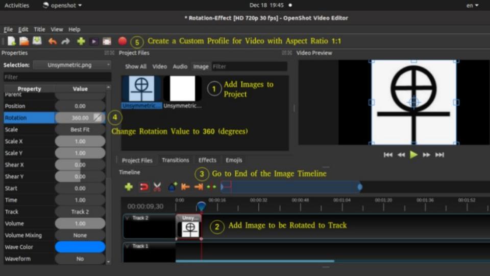
description=Aspect_ratio_1 - Name of new profile
frame_rate_num=30000       - Frame rate numerator
frame_rate_den=1000        - Frame rate denominator
width=310                  - Width of the video
height=310                 - Height of the video
progressive=1              - 1 = both even and odd rows of pixels used
sample_aspect_num=1        - Numerator of pixel shape aspect ratio
sample_aspect_den=1        - Denominator of pixel shape aspect ratio
display_aspect_num=16      - Numerator of display aspect ratio
display_aspect_den=9       - Denominator of display aspect ratio
The output shall look like as shown below. Note that when a square a rotated, its corners shall get trimmed as maximum dimensions (the diagonal) exceeds the width of the video.
In order to remove the corner-trimming effect while rotating an image, follow the steps described in image below.
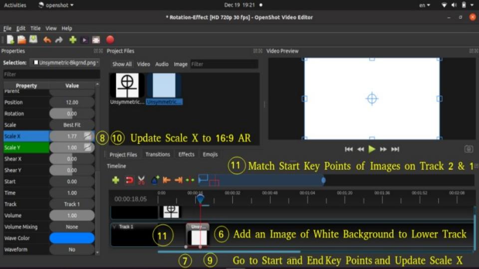
This rotation effectcan also be created using this code in Python and OpenCV.
OpenShot provides options to create 3D animation using Animated Titles menu. It requires another open source program Blender.
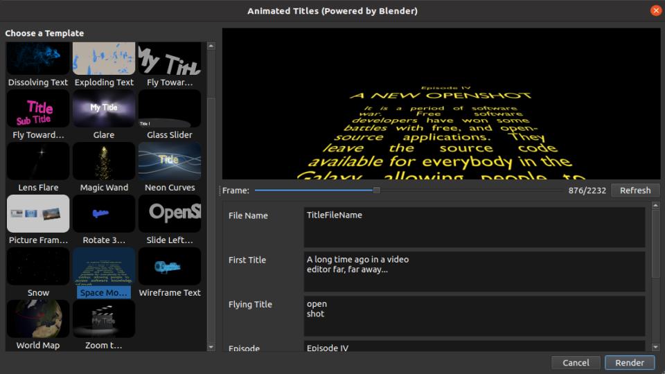
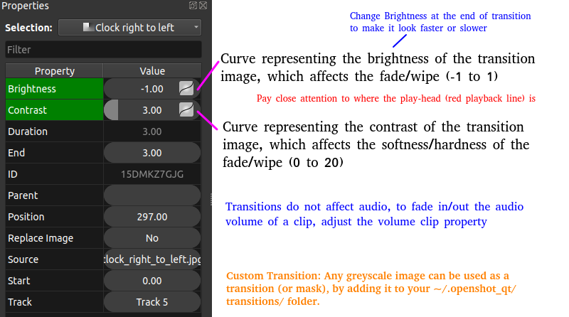
Making Corrections in the Videos: if you have misspelt certain words in a video and the frames contain background colour or image, adding the corrected text alone shall overlap with the incorrect text. One method which I use is to go back to the original source which was used to create the frame (for example a PowerPoint slide or Image where text was added manually or Title in an image editing program), create an image of the corrected text (word and/or string) and then overlay this image for the duration that wrong text appears in the video. This can be quickly done in OpenShot. If you have made grammatical errors in narration, not much options exist but to re-record that section.
Machine Learning in Image Data
How to detect if an image has been tampered or not? Same for videos? How to check if a video or image was created using AI/MP application or program? How to find if characters in a video are real?Markov Chain and Hidden Markov Models (HMM)
As per MathWorks Inc: Markov processes are examples of stochastic processes - processes that generate random sequences of outcomes or states according to certain probabilities.
Also known as "time series analysis", this model is in many aspects similar to Naive-Bayes model and in fact based on Bayes theorem. HMM is used to find a likely sequence of events for a given sequence of observations. Here the probability of a future event is estimated based on relative frequency of past observations of sequence of events (thus known prior probabilities). Probabilities to go from state 'i' to state 'i+1' is known as transition probability. The emission probability refers to the likelihood of of a certain observation 'y' when model is in state 's'.Markov Chain: P(En|En-1, En-1 ... E2, E1) = probability of nth event given known outcome of past (n-1) events.
First Order Markov Assumption: P(En|En-1, En-1 ... E2, E1) = P(En|En-1) that is probability of nth event depends only of known outcome of previous event. This is also known as "memoryless process" because the next state depends only on the current state and not on the chain of events that preceded it or led the latest state. This is similar to tossing a fair coin. Even if one gets 5 or 20 successive heads, the probability of getting a head in next toss is still 0.50.
Markov first order assumption may or may not be valid depending upon the application. For example, it may not be a valid assumption in weather forecasting and movement of stock price. However, it can be a valid assumption in prediction of on-time arrival of a train or a flight.
Trellis Diagram: This is a graphical representation of likelihood calculations of HMMs.
Example calculations:
- Suppose the initial or prior probabilities of 'clear' and 'foggy' day during December-January in northern part of India are: P(C) = 0.3, P(F) = 0.7.
- The transition probabilities are: P(C|C) = 0.2, P(C|F) = 0.1, P(F|F) = 0.6, P(F|C) = 0.5
- Probability of a sequence of states in this example say P({F, F, C, C}) = P(C|C) × P(C|F) × P(F|F) × P(F) = 0.2 × 0.1 × 0.6 × 0.7 = 0.0084
The following OCTAVE script implements a Gaussian model to detect anomalous examples in a given dataset. The Gaussian distribution is mathematically represented as follows. The data in a CSV file used for cross-validation can be downloaded from here.
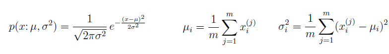
%----Ref: github.com/trekhleb/machine-learning-octave/anomaly-detection/--------
%Anomaly detection algorithm to detect anomalous behavior in server computers.
%The features measure the throughput (Mb/s) and latency (ms) of response of each
%server. m = 307 examples of how they were behaving, the unlabeled dataset. It
%is believed that majority of these data are normal or non-anomalous examples of
%the servers operating normally, but there might also be some examples of servers
%acting anomalously within this dataset. Label y = 1 corresponds to an anomalous
%example and y = 0 corresponds to a normal example.
clear; close all; clc;
%
%Load the data.
A = csvread("serverParams.csv");
X = [A(:, 1) A(:, 2)]; Y = A(:, 3);
%
%Estimate MEAN and VARIANCE: parameters of a Gaussian distribution
%Get number of training sets and features. size(X) returns a row vector with the
%size (number of elements) of each dimension for the object X. m=rows, n=cols
[m n] = size(X);
mu = mean(X);
s2 = (1 / m) * sum((X - mu) .^ 2);
%
%Visualize the fit
[X1, X2] = meshgrid(0 : 0.5 : 30);  U = [X1(:) X2(:)];
[m n] = size(U);
%
%Returns the density of the multivariate normal at each data point (row) of X
%Initialize probabilities matrix
Z = ones(m, 1);
%
%Go through all training examples and through all features. Returns the density
%of the multivariate normal at each data point (row) of X.
%
for i=1:m
  for j=1:n
    p = (1 / sqrt(2 * pi * s2(j))) * exp(-(U(i, j) - mu(j)) .^ 2 / (2 * s2(j)));
    Z(i) = Z(i) * p;
  end
end
Z = reshape(Z, size(X1));
%
%Visualize training data set.
plot(X(:, 1), X(:, 2),'bx'); hold on;
%
%Do not plot if there are infinities
if (sum(isinf(Z)) == 0)
  contour(X1, X2, Z, 10 .^ (-20:3:0)');
end
hold off;
xlabel('Latency (ms)'); ylabel('Throughput (MB/s)');
title('Anomaly Detection: Server Computers');
%
%Returns the density of the multivariate normal at each data point (row) of X
%Initialize probabilities matrix
[m n] = size(X); prob = ones(m, 1);
%
%Go through all training examples and through all features. Returns the density
%of the multivariate normal at each data point (row) of X.
for i=1:m
  for j=1:n
    p = (1 / sqrt(2 * pi * s2(j))) * exp(-(X(i, j) - mu(j)) .^ 2 / (2 * s2(j)));
    prob(i) = prob(i) * p;
  end
end
%
%Select best threshold. If an example x has a low probability p(x) < e, then it
%is considered to be an anomaly.
%
best_epsilon = 0;
best_F1 = 0;
F1 = 0;
ds = (max(prob) - min(prob)) / 1000;
prec = 0; rec = 0;
for eps = min(prob):ds:max(prob)
  predictions = (prob < eps);
  % The number of false positives: the ground truth label says it is not
  % an anomaly, but the algorithm incorrectly classifies it as an anomaly.
  fp = sum((predictions == 1) & (Y == 0));

  %Number of false negatives: the ground truth label says it is an anomaly, but
  %the algorithm incorrectly classifies it as not being anomalous.

  %Use equality test between a vector and a single number: vectorized way rather
  %than looping over all the examples.
  fn = sum((predictions == 0) & (Y == 1));

  %Number of true positives: the ground truth label says it is an anomaly and
  %the algorithm correctly classifies it as an anomaly.
  tp = sum((predictions == 1) & (Y == 1));

  %Precision: total "correctly predicted " positives / total "predicted" positives
  if (tp + fp) > 0
    prec = tp / (tp + fp);
  end
  %Recall: total "correctly predicted" positives / total "actual" positives
  if (tp + fn) > 0
    rec = tp / (tp + fn);
  end
  %F1: harmonic mean of precision and recall
  if (prec + rec) > 0
    F1 = 2 * prec * rec / (prec + rec);
  end

  if (F1 > best_F1)
    best_F1 = F1;
    best_epsilon = eps;
  end
end

fprintf('Best epsilon using Cross-validation: %.4e\n', best_epsilon);
fprintf('Best F1 on Cross-validation set:  %.4f\n', best_F1);

%Find the outliers in the training set and plot them.
outliers = find(prob < best_epsilon);

%Draw a red circle around those outliers
hold on
plot(X(outliers, 1), X(outliers, 2), 'ro', 'LineWidth', 2, 'MarkerSize', 10);
legend('Training set', 'Gaussian contour', 'Anomalies');
hold off
The output from the program is: 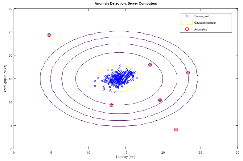
Recommender Systems and Collaborative Filtering
Collaborative filtering refers to the fact that contribution by each user by providing ratings to a product, book, music, brand, movie... etc help make a better rating system and in turn get a accurate rating for the product, brand, movie... for himself / herself. Users with ratings similar to a specific user 'A' is called neighbours of 'A'. All the ratings given by the user 'A' is called a "rating vector".Jaccard Similarity: similarity(A, B) = |rA ∪ rB| / |rA ∩ rB| where rA and rB are rating vectors for users A and B respectively. Thus: similarity(A, B) = total common ratings / total cumulative ratings. It ignores the rating values and is based solely on number of ratings by the users.
Cosine Similarity: similarity(A, B) = cos(rA, rB) which is similar to the dot product of vectors. Thus: similarity(A, B) = Σ[rA(i).rB(i)] / |rA| / |rA|. It treats the blank entries (missing values) in rating vector as zero which is counter-intuitive. If a user did not rate a product does not mean he/she strongly dislikes it.
Centred Cosine Similarity: This is very much similar to cosine similarity and is also known as Pearson Correlation. However, the rating vector for each user is "normalized about mean". Thus, r'A(i) = rA - [Σ(rA(i)]/N. similarity(A, B) = cos(r'A, r'B). It still treats the blank entries (missing values) in rating vector as zero which is average rating (note mean = 0). It handles the effect or bias introduced by "tough raters" and "easy raters" by normalizing their rating values.
Item-Item collaborative filtering refers to method of filtering based on ratings for items (books, movies...) by all users. User-User collaborative filtering refers to method of filtering based on all ratings by a user for items (books, music, movies...). Though both of these approach looks similar, the former performs significantly better than the later in most use cases. However, note that it is important to take care of user which has not rated any item than the item which has not got any rating. An item which has not been rated does not any way qualify for any recommendations to any user.Example: Given the rating for 8 movies by 9 users, estimate the rating of movie 'B' by user '3'.
| Movies | Users and their ratings | Rating vector | ||||||||
| 1 | 2 | 3 | 4 | 5 | 6 | 7 | 8 | 9 | ||
| A | 3.0 | 4.0 | 1.0 | 2.0 | 3.0 | 5.0 | rA | |||
| B | 2.0 | ? | 2.0 | 3.0 | 4.0 | rB | ||||
| C | 4.0 | 4.0 | 1.0 | 3.0 | 2.0 | rC | ||||
| D | 2.0 | 3.5 | 4.0 | 3.0 | 4.0 | rD | ||||
| E | 3.0 | 2.0 | 5.0 | 5.0 | 1.0 | 3.5 | rE | |||
| F | 2.0 | 1.0 | 4.0 | 3.0 | 5.0 | rF | ||||
| G | 1.0 | 2.0 | 3.0 | 4.0 | 2.0 | rG | ||||
| H | 1.0 | 2.0 | 3.0 | 2.0 | 5.0 | rH | ||||
Step-1: Normalize the ratings about mean zero and calculate centred cosine. In MS-Excel, one can use sumproduct function to calculate the dot product of two rows and columns. Thus: rA . rB = sumproduct(A1:A9, B1:B9) / sqrt(sumproduct(A1:A9, A1:A9)) / sqrt(sumproduct(B1:B9, B1:B9)).
| User | Users and their ratings after mean normalization | s(X, B): X = {A, B, C ... H} | ||||||||
| 1 | 2 | 3 | 4 | 5 | 6 | 7 | 8 | 9 | ||
| A | 0.000 | 1.000 | -2.000 | -1.000 | 0.000 | 2.000 | 0.000 | |||
| B | -0.750 | ? | -0.750 | 0.250 | 1.250 | 1.000 | ||||
| C | 1.200 | 1.200 | -1.800 | 0.200 | -0.800 | 0.012 | ||||
| D | -1.300 | 0.200 | 0.700 | -0.300 | 0.700 | 0.162 | ||||
| E | -0.250 | -1.250 | 1.750 | 1.750 | -2.250 | 0.250 | -0.063 | |||
| F | -1.000 | -2.000 | 1.000 | 0.000 | 2.000 | 0.048 | ||||
| G | -1.400 | -0.400 | 0.600 | 1.600 | -0.400 | -0.026 | ||||
| H | -1.600 | -0.600 | 0.400 | -0.600 | 2.400 | 0.328 | ||||
Step-2: For assumed neighbourhood of 3, find the 3 movies which has been rated by user 'B' and similarity s(X,B) is the highest in s(X,B) vector. Thus, movie A, D and H which are rated by user '3' and their similarities are highest among s(X,B).
Step-3: Use similarity weights and calculate weighted average. Similarity weights: s(C,B) = 0.012, s(D,B) = 0.162, s(H,B) = 0.328. Likely rating of movie by user '3' = weighted average calculated as follows.
r(B, 3) = s(C,B) . r(C,3) + s(D,B) . r(D,3) + s(H,B) . r(H,3) / [s(C,B) + s(D,B) + s(H,B)] = (0.012 * 4.0 + 0.162 * 3.5 + 0.328 * 2.0) /(0.012 + 0.162 + 0.328) = 2.53
The following code is an improvisation of GNU OCTAVE script available on gitHub. There are many versions of this scripts uploaded there. The movie rating data in CSV (zip) format can be downloaded from here. Other functions are available here: fmincg.m, collaborative filtering coefficients and movie id / name. This script is for demonstration only and not fully debugged: the predicted rating is higher than 5 which is not correct.
% -----------------------Movie Recommender using GNU OCTAVE / MATLAB -----------
clc; clear;
%
%Load data from a CSV file: first half contains rating and later half ON/OFF key
A = csvread("movieRatings.csv");
[m2, n] =  size(A); m = m2 / 2;
%
%Split the matrix A into user rating matrix 'Y' and  1/0 matrix 'R'
Y = A([1:m], :); R = A([m+1:m2], :);
%
%Find out no. of non-zero elements (actual number of ratings) in each row
Yc = sum(Y ~= 0, 2);
fprintf('\nHighest number of ratings received for a movie: %d \n', max(Yc));
%
% Read the movie list
fid = fopen('movie_ids.txt');
g = textscan(fid,'%s','delimiter','\n');  n = length(g{1}); frewind(fid);
movieList = cell(n, 1);
for i = 1:n
  line = fgets(fid); % Read line
  [idx, mName] = strtok(line, ' '); %Word Index (ignored since it will be = i)
  movieList{i} = strtrim(mName);   % Actual Word
end
fclose(fid);
%
%Initialize new user ratings
ratings = zeros(1682, 1);
%
%return
%Stop execution and return to command prompt - useful for debugging
%
% Y = 1682x943 matrix, containing ratings (1-5) of 1682 movies by 943 users
% R = 1682x943 matrix, where R(i,j) = 1 if user j gave a rating to movie i
% q(j) = parameter vector for user j
% x(i) = feature vector for movie i
% m(j) = number of movies rated by user j
% tr(q(j)) * x(i) = predicted rating for user j and movie i
%
fprintf('\n Training collaborative filtering...\n');
%
%Estimate mean rating ignoring zero (no rating) cells
Ym = sum(Y, 2) ./ sum(Y ~=0, 2);
%
%Mean normalization
Yn = Y - Ym .* (Y ~= 0);
%
%mean(A,2) is a column vector containing the mean of each row
%mean(A) a row vector containing mean of each column
%
%Get data size
n_users    = size(Y, 2);
n_movies   = size(Y, 1);
n_features = 10;         %e.g. Romance, comedy, action, drama, scifi...
ratings    = zeros(n_users, 1);
%
%Collaborative filtering algorithm
%Step-1: Initialize X and Q to small random values
X = randn(n_movies, n_features);
Q = randn(n_users, n_features);    %Note Q (THETA) and q (theta) are different
q0 = [X(:); Q(:)];
%
%Set options for fmincg
opt = optimset('GradObj', 'on', 'MaxIter', 100);
%
%Set regularization parameter
%Note that a low value of lambda such as L = 10 results in predicted rating > 5.
% However, a very high value say L=100 results in high ratings for those movies
% which have received only few ratings even just 1 or 2.
L = 8;
q = fmincg (@(t)(coFiCoFu(t, Yn, R, n_users, n_movies, n_features, L)), q0,opt);
%
% Unfold the returned theta matrix [q] back into X and Q
X = reshape(q(1 : n_movies * n_features), n_movies, n_features);
Q = reshape(q(n_movies * n_features + 1:end), n_users, n_features);
%
fprintf('Recommender system learning completed.\n');

%Make recommendations by computing the predictions matrix.
p = X * Q';
pred = p(:,1) + Ym;
%
[r, ix] = sort(pred, 'descend');
fprintf('\n Top rated movies:\n');
for i=1:10
  j = ix(i);
  fprintf('Predicting rating %.1f for %s, actual rating %.2f out of %d\n', ...
    pred(j), movieList{j}, Ym(j), Yc(j));
end
Reinforcement Learning - RL
It is behavioral learning model which differs from other types of supervised learning methods because the system is not trained with the any labelled data set. This is a training algorithm based on 'rewards' and 'penalties' of an action. Like a child when on falls over a slippery (wet) surface, next time when someone has to cross such surface, he/she will use his/her toes to improve the grip and increase grip as the smoothness of the surface is felt. In RL, the terms agent, environment, reward, penalty and policy are most frequently used concepts. While in an organization, policy refers to a set of guidelines, templates, forms and workflows, in RL policy is a deep neural network (NN) which decides actions taken by the agent. The gaming program AlphaGo is based on RL algorithm. It can be applied in motion controls of a robotic arms to grasp and move items.While training a robot to balance itself while walking and running, the RL training algorithm cannot let it fall and learn, not only this method will damage the robot, it has to be picked and set upright every time it falls. Reinforcement learning is also the algorithm that is being used for self-driving cars. One of the quicker ways to think about reinforcement learning is the way animals are trained to take actions based on rewards and penalties. Do you know how an elephant is trained for his acts in a circus?
Q-Learning algorithm: this is based on Bellman equation [Q(s,a) = sT.W.a], where {s} is states vector, {a} denotes actions vector and [W] is a matrix that is learned] which calculates "expected future rewards" for given current state. The associated data is Q-table which is a 2D table with 'states' and 'actions' as two axes.Natural Language Processing (NLP)
Adapted from "Machine Learning For Dummies, IBM Limited Edition": NLP is the ability to train computers to understand both (hand-written and typed) text and human speech (voice). NLP techniques are needed to capture the meaning of unstructured text from documents or communication from the user. Therefore, NLP is the primary way that systems can interpret text and spoken language. NLP is also one of the fundamental technologies that allows non-technical people to interact with advanced technologies. For example, rather than needing to code, NLP can help users ask a system questions about complex data sets. Similarly, a user can develop his own website without knowing much about HTML and css. Unlike structured database information that relies on schemas to add context and meaning to the data, unstructured information must be parsed and tagged to find the meaning of the text. Tools required for NLP include categorization, ontologies, tapping, catalogues, dictionaries and language models.Model Selection Criteria
As evident in methods and programs outlined above, machine learning is about "selection of models and parameters". Field of information theory is used to quantify or measure the expected value of information - various goodness-of-fit tests have been developed to assess the performance of a model with respect to how well it explains the data. Akaike information criterion (AIC) is considered the first model selection criterion that is appropriate to be used in practice where the best model is the candidate model with the smallest AIC.Another criterion, the Bayesian information criterion (BIC) was proposed by Schwarz (also referred to as the Schwarz Information Criterion - SIC or Schwarz Bayesian Information Criterion - SBIC). This is a model selection criterion based on information theory which is set within a Bayesian context. Similar to AIC, the best model is the one that provides the minimum BIC. [Reference: www.methodology.psu.edu/resources/aic-vs-bic] AIC is better in situations when a false negative finding would be considered more misleading than a false positive. BIC is better in situations where a false positive is as misleading as or more misleading than a false negative.
One of the method to validate a model is known as "k-fold cross validation" which can be described as shown in following image.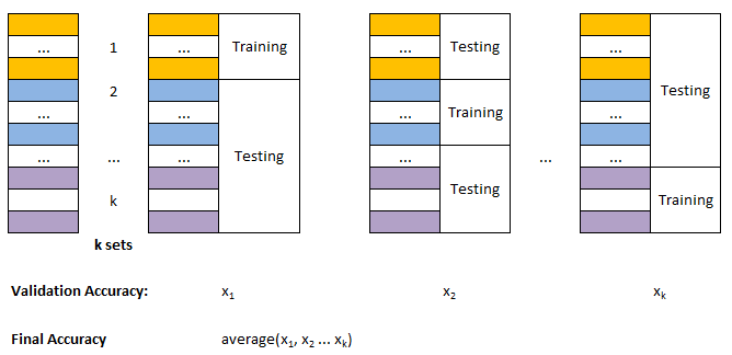
AI - The Unknown Beast!
AI has already started affecting my decisions and impulses. When I search for a flight ticket, related ads start appearing. I believe that fare starts increasing when I make many searches before actually booking and Uber or Ola cab. On the hindsight, so far none of the ads which pop-up through Google ads have helped me because they appear when I have already made the purchase or have pushed the buying decision for future months. Also, most of the ads appear not when I am interested to buy them but want to understand the technology behind them. Based on my browsing history and interest, the accuracy of ads shown by google is not more than 5%.I have certainly used the recommendations generated by youTube and viewed many videos based on their recommendations. Though I found them useful, there was nothing extra-ordinary in those recommendations.
One of the possible problem I see is the integrity and authenticity of data/information. I have come across many videos on youTube which are either too repetitive or fake or even factually incorrect. I have heard how AI can diagnose the disease from X-rays and CT-scans. In my opinion, an expert or experience doctor can identify the issue from naked eyes within seconds. These tools are going to make even a naive doctor look like expert! Hence, the AI may help incompetent doctors. How this capability is going to address the patient remains unanswered - will it lead to lesser consultation fee and/or lesser waiting time?
AI tools can also be considered having implications similar to "dynamite and laser". These are used for constructive purposes such as mining and medical diagnosis whereas dangerous aspects like "bomb blasts and laser-guided missiles" are also known. Is AI going to make "forensic expert's" life easy or tough? Is it going to introduce significant biases in the virtually opaque implementations in customer segmentations?
Identity Theft: E-mail address hunting, Reverse image search, Social Media post scraping, whois service of a website: reveals complete information (phone number, e-mail ID, residential address) if privacy protection is not enabled or purchased. OSINT: Open Source INTelligence is a way to gathering information from social media using usernames.
In the name of company policy, none of the social media platform publish (and shall publish) even a partial list of rules used by them to filter and delete/ban posts on their websites. This complete opaque implementation of AI tools is a lethal weapon to mobilize resources to affect public opinion and influence democratic processes. There are posts and videos on YouTube that threaten about annihilation of particular community. There are videos still up (as in Dec-2022) where a preacher claims Right of Islam to kill non-muslims and especially few special categories of non-muslims. However, the AI tool is configured such that anybody posting against that video content with same level of pushback (such as non-muslims also have right to kill muslims) shall get suspended from the platform. I firmly believe that any expectation that AI can be used to make the communication balanced, open and honest is just a wishful thinking - AI has created potential to make it more biased and one-sided than traditional modes.
Deep Learning
Python, TensorFlow and Keras: TensorFlow derives its name from "operations on tensors" where a tensor is a multi-dimensional array. It contains deep learning libraries which include those from Keras.Following sections of this page provides some sample code in Python which can be used to extract data from web pages especially stock market related information. Sample code to generate plots using matplotlib module in Python is also included.
Web Scraping in Python
The term web scraping refers to collecting information from web sites. However, the same concept can be used to check the consistency and correctness of tags and links in folder structure of a website before uploading the content on host server. If a website fetches data using Javascript (called Dynamic pages such as nseindia.com), requests and urllib libraries cannot be used. These tools work only for static pages (where the contents are directly stored in HTML page being accessed).import re
def split_string_at_numbers(input_string):
# Check for +/- sign, digits, decimal point
pattern = r'(-?\d+\.?\d*|\d*\.?\d+)'
# Split the string by the number pattern, keeping delimiters
sub_str = re.split(pattern, input_string)
sub_str_txt = []
sub_str_num = []
for str_txt in sub_str :
if str_txt:
try:
num = float(str_txt)
if num == int(num):
sub_str_num.append(int(num))
else:
sub_str_num.append(num)
except ValueError: # If conversion fails, it implies a string
sub_str_txt.append(str_txt)
for item_txt, item_value in zip(sub_str_txt, sub_str_num):
#print(f"{item_txt} | {item_value}")
print('{} | {}'.format(item_txt, item_value))
return sub_str_txt, sub_str_num
This Python code is a simple and scalable example to check the image tags in all the HTML files stored in a folder and print summary of image tags such as relative path of image file, its file size, missing images...This code can be further improvised to include HREF tags, missing ALT tag for images, add styles to the images, remove styles of the images such as width and height... to name a few.
Python code lined here is a simple and scalable example to check the <a> tags and HREF values in all the HTML files stored in a folder and print summary of hyperlinks such as relative path of the file referred by HREF, missing files in the links... This code does not check the hyperlinks referred by HREF starting with http or https. This script can be further improvised to check for missing attribute values such as _blank.
Pandas
Print each column name as rowfor col_name in DataFrame.columns.to_numpy(): print(col_name).
DataFrame                                <- = Table
   col_1 | col_2 | col_3 | ... | col_N   <- Column Labels or Series

0   v_11 |  v_12 |  v_13 | ... |  v_1N   <- DataFrame.loc[0] `] df.loc[0: 2]
1   v_21 |  v_22 |  v_23 | ... |  v_2N   <- DataFrame.loc[1]  ]   or
2   v_31 |  v_32 |  v_33 | ... |  v_3N   <- DataFrame.loc[2] _] df.loc[0,1,2]
.
.
.
Tips and Tricks on Handling Devices
- If you want to transfer data from one device (say computer) to another device (say mobile or external hard disk), either ZIP the source files or transfer one folder (few files) at a time. Copy-paste function on large number of files (say > 10,000) slows down the data transfer speed.
- In case you want to cut-paste some data, it is safer to use copy-paste and then delete the source data after the file transfer is successful.
- Like in previous case if you want to replace some data, it is safer to rename the destination folder and delete once data transfer is complete. An overwrite operation cannot be corrected (which files were overwritten) if there is any error during the process.
- The Print Screen key does not work when some pop-up or sub-menu window is open in a Program. In Ubuntu Linux, Screenshot application with delay can be used to capture window in such cases. Turn the Screenshot with 5 seconds delay as shown below, click "Take Screenshot" tab, go to the program where a sub-menu needs to be open, wait for set number of seconds for screen to get captured.
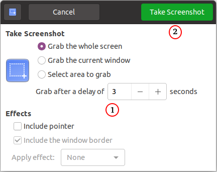
Edit epub Files
EPUB files are structurally a compressed (ZIP) file containing XHTML text files, images, and other resources. To unzip the epub to the folder 'eBook': "unzip eBbook.epub -d eBook". To zip up an epub, follow the following steps. Note that the option -r stands for recursive operation and -g is needed to add additional files (grow) to interim zip folder.- zip -X newEbook.epub eBook/mimetype
- zip -rg newEbook.epub eBook/META-INF -x \*.DS_Store
- zip -rg newEbook.epub eBook/OEBPS -x \*.DS_Store
Calibre
This package can be used to view, edit and convert ePUB files. The Calibre install provides the command ebook-convert that runs from command line and there's no need to run Calibre. For example: "ebook-convert eBook.epub eBook.pdf --enable-heuristics" can be used to convert a EPUB file to PDF. Multi-column PDFs are not supported and this command line operation shall not work, only way left is to edit the PDF in GUI mode.
MoviePy Functions Tested in Ubuntu 20.04 LTS

MoviePy as described earlier is a wrapper around FFmpeg to edit videos and audios. This file contains few functions which can be used to create freezing frame effects and trim unwanted frames from videos. This code can be used to add text to a blank video. Attempts were made to improvise the example scripts available in the official documentation, many of them did not work and the error were too cryptic to debug.
This code to create End Effect is adapted from example scripts provided in documentation.
 FAQ: OpenShot
Q01: How are the effects created?
A01: Effects are created by combination of following attributes or features: location, position, rotation, scale, scale X, scale Y, shear X, shear Y, brightness, Transparency...
Q02: How can a video be masked?
A02: A video mask is create using Alpha or Transparency value of the video clip and that of the mask object
Q03: How can a text be added to a video?
A03: A text is added using Title options in OpenShot. Title may look to have black background but it is a transparent background. Any image can be used to change the background colour of the title. Also, there is an option to use title of type "Solid Color" and the background can be selected to any pre-defined colours.
Q04: How can a horizontal or vertical line be drawn?
A04: Use a title of solid colour -> change Scale Y to 0.05 for horizontal line or Scale X to 0.05 for vertical line.
Q05: Can a scrolling text be added to a video?
A05: Yes, a scrolling text [or an image with required text] from left-to-right or right-to-left can be added using a text box and changing the position of the text box from extreme right [at start of the video or at any time frame after start] to extreme left [at end of video or any time frame before the end].
Q06: Can the typewriter effect be created in OpenShot?
A006: No as on version 3.1.1. A more tedious and even impractical way it to create title for each character.
Q07: How can one type in non-Roman script say Devanagari (Hindi)?
A07: Using 'Advance' editor. You need to get the text in desired script from other sources such as Google Translate. Copy paste that non-Roman script inside the Inkscape window which open once you click on "Use Advance Editor".
Q08: Can a screen pump (temporary zoom-in) effect be created?
A08: Yes, you just need to adjust the scale value near the time frame you want to create Zoon-in effect.
Q09: Can the Camera Flash effect be created in OpenShot?
A09: Yes, use transparency (alpha) value of the clip.
Q10: Can a video or image be mirrored in OpenShot?
A10: Yes, use scale X = -1 to flip or mirror the video in horizontal direction and scale Y = -1 for vertical direction
Q11: Can a video play behind an image?
A11: Yes, set transparency (alpha) value of the image to < 1 typically in the range 0.4 ~ 0.5
Q12: Can a video be played faster or slower?
A12: Yes, right click on the clip -> Time -> Slow -> Forward -> 1/2X or 1/4X or 1/8X or 1/16X. Note that the overall duration of video is increased in same proportion.
Q13: How can the Paint Effect of Character Introduction effect be created in OpenShot?
A13: Split the clip at desired time, Right click on the clip -> Time -> Freeze or Freeze and Zoom. Note that the duration of the clip is increased by Freeze time selected.
 Video Editing using Blender
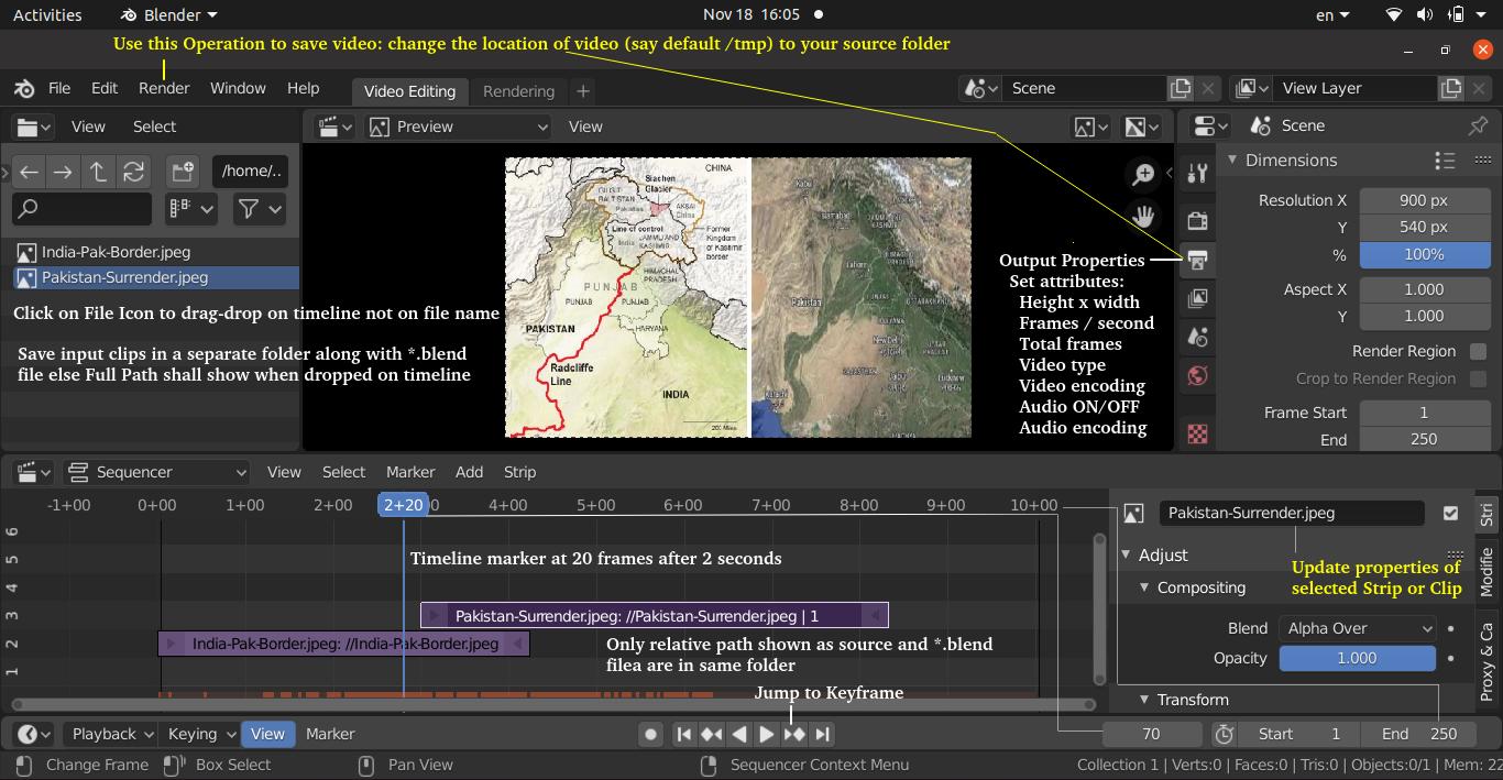
Adding Effects & Transitions: To add an effect strip, select one base strip (image, movie, or scene) by clicking MB1 on it. For some effects, like the Cross transition effect, use Shift-LMB to select a second overlapping strip. From 'Add' menu pick the effect to be created and the 'Effect' strip will be shown above the source strips.
In the video strips, strip name, path to source file, and strip length are shown. For image strips, the strip length is fixed to 1.
Alpha Over: With Alpha Over, the strips are layered up in the order selected; the first strip selected is the background, and the second one goes over the first one selected. The Opacity controls the transparency of the foreground, i.e. Opacity of 0.0; will only show the background, and an Opacity of 1.0 will completely override the background with the foreground. Alpha Under: the first strip selected is the foreground, and the second one, the background.
Creating a Slow-Motion Effect: To slow strip down the video clip without affecting the overall frame rate, select the clip and Add > Effect > Speed Control effect strip.
Wipe Strip: The Wipe transition strip is used to transition from one strip to the next: duration of the wipe is the intersection of the two source strips and cannot be adjusted. To adjust the start and end of the wipe, temporal bounds of the source strips should be adjusted in a way that alters their intersection.
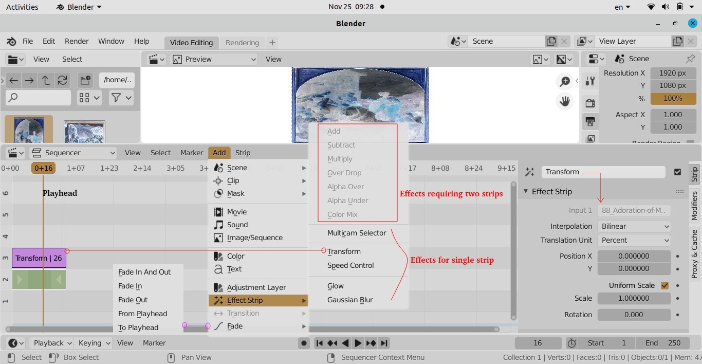
Other products offering similar features are Maya 3D and Houdini. From the website of Autodesk: "What is Maya? Maya is professional 3D software for creating realistic characters and blockbuster-worthy effects. Bring believable characters to life with engaging animation tools. Shape 3D objects and scenes with intuitive modelling tools. Create realistic effects – from explosions to cloth simulation." From the official page of Houdini: "Houdini is built from the ground up to be a procedural system that empowers artists to work freely, create multiple iterations and rapidly share workflows with colleagues. In Houdini, every action is stored in a node. These nodes are then “wired” into networks which define a “recipe” that can be tweaked to refine the outcome then repeated to create similar yet unique results. The ability for nodes to be saved and to pass information, in the form of attributes, down the chain is what gives Houdini its procedural nature." ANSYS Discovery has on option called Vectorize Image that creates curves around colored areas in images.
PowerBI and Pivot Tables
Excerpt from Microsoft website about PowerBI: Find insights in your data and share rich analytics reports. Explore your reports to find and generate the quick insights you need for better business decisions. Collaborate on reports with colleagues, then easily share reports and insights in workspaces, on the web, in apps, via Microsoft Teams.How to Create a Pivot Table
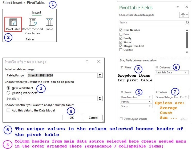
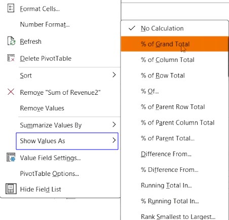

Cursor AI
Tag line on official website: "The AI Code Editor". More from website: "Cursor lets you write code using instructions. Update entire classes or functions with a simple prompt. Cursor's agent mode completes tasks end to end. It does this quickly, while keeping programmers in the loop. We support all frontier coding models, including Claude Sonnet 4, OpenAI o3-pro, OpenAI GPT-4.1, Gemini 2.5 Pro, Claude Opus 4, and more."Thus, Cursor AI is a code editor that uses artificial intelligence models to help code writers with coding tasks such as code generation, smart rewrites, codebase queries and end-to-end task completion.
The content on CFDyna.com is being constantly refined and improvised with on-the-job experience, testing, and training. Examples might be simplified to improve insight into the physics and basic understanding. Linked pages, articles, references, and examples are constantly reviewed to reduce errors, but we cannot warrant full correctness of all content.
Template by OS Templates