- CFD, Fluid Flow, FEA, Heat/Mass Transfer: Multi-phase Flows
OpenFOAM: Multiphase
Multi-phase Flow in OpenFOAM
Multi-phase Flows and Discrete Phase Models
Multi-phase flows have wide applications in process, refrigeration, air conditioning, petroleum, oil and gas, food processing, automotive, power generation and metal industries including phenomena like mixing, particle-laden flows, CSTR - Continuously Stirred Tanks Reactor [gas dispersion and floating particles suspension in an agitated or stirred vessel], Water Gas Shift Reaction (WGSR), fluidized bed, fuel injection in engines, bubble columns, mixer vessels, Lagrangian Particle Tracking (LPT). Some of the general characteristics and categories of multi-phase flow are described below before moving to actual application of OpenFOAM utilities.
In a multiphase flow, the interface between the phases are influenced by motion of fluid. For example, water flowing through packed bed of rocks is a single phase flow. Multiphase flow regimes are typically grouped into five categories: gas-liquid (which are naturally immiscible) flows and (immiscible) liquid-liquid flows, gas-solid flows, liquid-solid flows, three or more phase flows. As can be seen, the immiscibility is a important criteria. In a multi-phase flow, one of the phase is usually continuous (carrier phase) and the other phase(s) are dispersed in it.
The adjective "Lagrangian" indicates that it relates to the phenomena of tracking a moving points ("fluid particles") - such as tracking a moving vehicle on a road. On the other hand, the adjective "Eulerian" is used to describe correlations between two fixed points in a fixed frame of reference - such as counting the type of vehicles and their speeds while passing through a fixed point on the road.
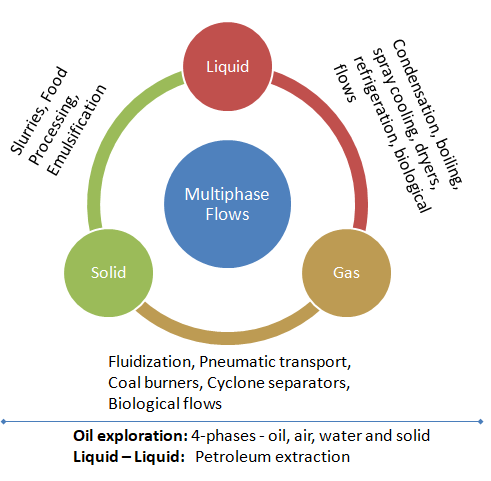
Gas-liquid flows are further grouped into many categories depending upon the distribution and shape of gas parcels. Three such types namely bubly, slug and annular are described in later paragraphs. Another broad classification of multiphase flows are 'homogeneous' and 'inhomogeneous'. The differences are tabulated below.
| Homogeneous Multiphase Flows | Inhomogeneous Multiphase Flows |
| All phases move at same velocity, same flow field | Each phase has its own flow field |
| There is no velocity 'slip' | There is velocity 'slip' |
| There is no interphase mass and momentum transfer | Interphase mass and momentum transfer are considered |
| Mixture momentum equation: momentum transfer between phases is assumed to be very large | Momentum equations for each phase: interfacial forces** acting on each phase causes momentum transfer |
| Mixture continuity equation | Continuity equations for each phase |
| Homogeneous pressure field* | Homogeneous pressure field |
| Homogeneous turbulence field | Homogeneous or inhomogeneous turbulence field |
The homogeneous model is also known as "friction factor" or "fog flow" model where two-phase flow is considered as single phase flow possessing mean flow properties. Note that the inhomogeneous model is not same as separated flow model. In the latter, the two phases are 'artificially' segregated into separate flow streams, one each for liquid and gas phases. In its basic form, each stream is assumed to flow at mean velocity. If the mean velocities of the two phases are equal, the separated flow model is equivalent to homogeneous model.
** the forces indicated are interphase drag force, lift force (perpendicular to the direction of relative motion of the two phases), wall lubrication force (tends to push the dispersed phase away from the wall), virtual mass force (proportional to relative phasic accelerations), interphase turbulence dispersion force and solids pressure force (for dense solid particle phases only).
The two dominant method of multi-phase simulations are listed below.
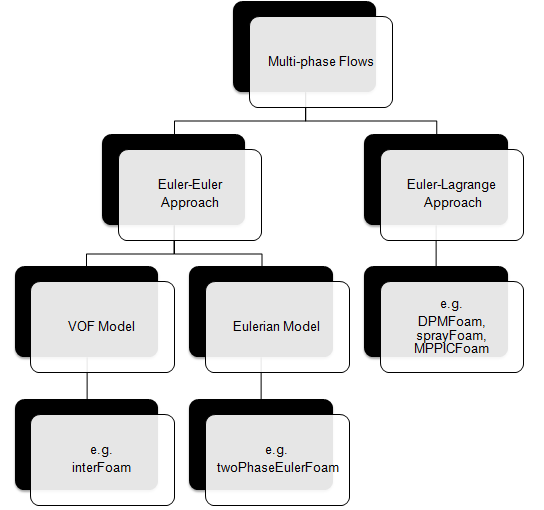
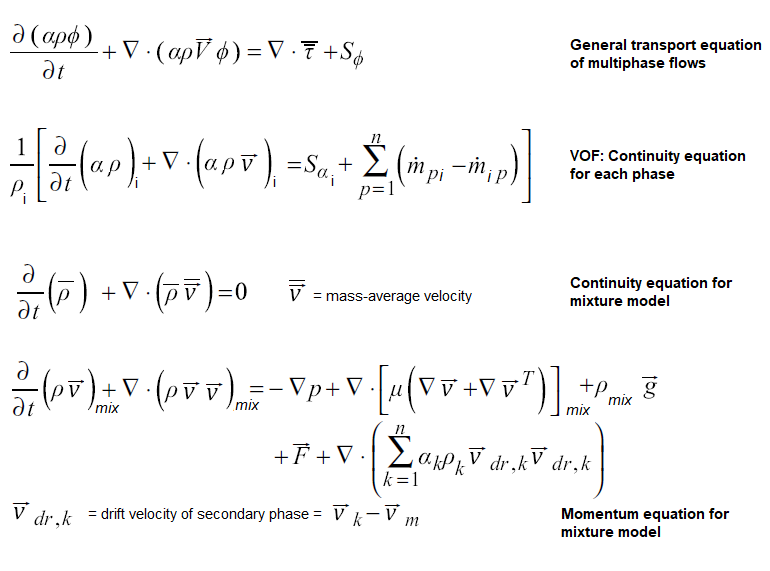
- VOF Model: it is a surface-tracking technique designed for two or more immiscible fluids where the position of the interface between the fluids is of interest. In this model, a single set of momentum equations is shared by the fluids, and the volume fraction of each of the fluids in each computational cell is tracked throughout the domain. Example applications of VOF model are filling and emptying of tanks or bottles, modeling of liquid splashing, sloshing inside a partially filled tank...
- Mixture Model: the phases are treated as interpenetrating continua and solves momentum equation for the mixture and prescribed relative velocities to describe the dispersed phases (but it can also be used without relative velocities for the dispersed phases to model homogeneous multiphase flow). It is a good substitute for the full Eulerian multiphase model (it can perform a full multiphase simulation while solving a smaller number of variables than the Eulerian approach and it is less computationally expensive compared to the Eulerian approach. In this case the momentum, continuity and energy equations for the mixture, the volume fraction equations for the secondary phases and algebraic expressions for the relative velocities are solved simultaneously. The essential approximation is the local equilibrium assumption which states that the particles are accelerated instantaneously to the terminal velocity. An algebraic formulation is used for the slip velocity which is based on the assumption of reaching to a local equilibrium between the phases over a short spatial length scale.
- Eulerian Model: the phases are treated as interpenetrating continua and a set of momentum and continuity equations for each phase are solved. Then the coupling is achieved through the pressure and interphase exchange coefficients. Application includes simulations of fluidized bed, mixing of immiscible fluids... Euler-Euler approach sometimes become a necessity such as cases like evaporation and condensation where heat and mass transfer between phases occur. In order to model heat transfer between the phases, separate enthalpy equations needs to be solved for each phase. This is possible only in Eulerian approach.
Excerpts from user manual for ANSYS FLUENT: "The VOF model is appropriate for stratified or free-surface flows and the mixture and Eulerian models are appropriate for flows in which the phases mix or separate and/or dispersed-phase volume fractions exceed 10%. (Flows in which the dispersed-phase volume fractions are ≤ 10% can be modeled using the discrete phase model)."
Mixing of Solid Particles
In many applications the mixing of solid particles of different sizes needs to be ensured such as cement powder and sand particles. Such simulations are carried out using DEM (Discrete Element Method) approach. LIGGGHTS [LAMMPS Improved for General Granular and Granular Heat Transfer Simulations] is an open-source Discrete Element Method particle simulation software based on LAMMPS - a classical molecular dynamics simulator.Mixing of Gases
The mixing of gases has many applications such as thermal comfort modeling, gas-stoves or burners, rotary kiln incinerators, dispersion of flue gases, smoke detection, hazardous gas such as refrigerant and hydrogen leak detection. An improvement of just a few percent in mixing efficiency can substantially reduce the energy consumption and emissions of a low-NOx burner. In bio-medicines, nasal sprays, gas mixing in respiratory tracts (airways) affects the performance of aerosolized medications.Condensation Simulation
Condensation is the change of the physical state of matter from gas phase into liquid phase. Latent heat effects associated with the phase change (enthapy of condensation) are significant higher than sensible heat effects (change in energy associated with change in temperature). Note that the enthalpy of condensation of water vapour at 0.101 MPa (atmospheric pressure) is Δh = – 2257 [kJ/kg]. There are 3 types of condensation mechanism as described below. Interphase heat transfer occurs due to thermal non-equilibrium across phase interfaces.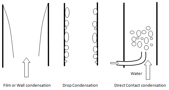
- Wall or Film Condensation: In this process, the condensing steam (vapour) forms film layer on the wall surface which needs to be modeled as mass transfer phenomena from the gas (vapour) phase to the liquid phase in the near wall grid cells. The heat transfer from the vapour phase away from the wall though the wall film to the wall needs to be resolved. Since, there is an interface between the vapour (gas) and liquid phase, it (the phase interaction) needs to be modeled explicitly (say using UDF in ANSYS FLUENT) and cannot be a natural outcome of energy equations of each phase.
- Drop-wise condensation: it takes place when the surface over which condensation occurs is non wet-able (e.g. surface coatings with silicons, teflons or waxes). In this mode, when steam condenses, the droplets are formed. When the drops become bigger, they simply fall under the gravity. In drop wise condensation, high heat transfer rates are achieved.
- Direct Contact Condensation or Bulk Condensation: the vapor is brought into direct contact with a liquid at a temperature below the saturation temperature of the vapour. E.g. in jet condensers, the cooling water is sprayed on the exhaust steam and there is direct contact between the exhaust steam and cooling water. The reverse process is also adopted to heat up liquid by injecting stream directly into the liquid pipes. In CFD simulations of the direct-contact condensation, the challenges are in the estimation of the interfacial surface area, the heat transfer coefficient and interfacial drag in the different regions.
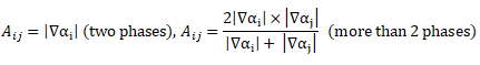
Interfacial transfer of momentum, heat and mass is dependent on the contact surface area between the two phases. This is characterized by the interfacial area per unit volume between phase and phase Aij, known as the interfacial area density which has dimensions of [m-1] or [1/length].
Total volume = 1 [unit] e.g. 1 [m3]. Volume of pahse 'j' = αj [m3].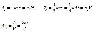

Since condensation processes require modeling of heat and mass transfer across the liquid - vapour interfaces. Since, interfaces are not well-defined shapes and cells cannot be fine enough to capture the interfaces precisely, different models have evolved to estimate condensation rate. One such widely used model is as per Lee.
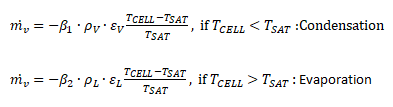
Since condensation is inherently a multi-phase phenomena, the CFD simulation approach comprise of modeling the mass transfer and heat transfer in multi-phase flow. ANSYS Fluent adds (source/sink terms) contributions due to mass transfer (mass transfer rate per unit volume) only to the momentum, species and energy equations. No source term is added for other scalars such as turbulence or user-defined scalars.
The volumetric rate of energy transfer between phases is assumed to be a function of the temperature difference and the interfacial area, Qij = hij × AINTERFACE × (Ti - Tj), where = hij is the volumetric heat transfer coefficient between the phases i and j. ANSYS FLUENT provides many option to model the interfacial heat transfer hij. They are Constant, Nusselt Number, Ranz-Marshall Model, Tomiyama Model (applicable to turbulent bubbly flows with relatively low Reynolds number), Hughmark Model (extends the Ranz-Marshall model to a wider range of Reynolds numbers), Gunn Model (for granular flows) and Two-Resistance Model.
Buoyancy in Multi-phase Flows
The difference in density between phases produces a buoyancy force in multiphase flows (including particle tracking). Hence, buoyancy is almost always play significant role in multiphase flows. For multiphase flows, it is important to correctly set the buoyancy reference density. For a flow containing a continuous phase (say water) and a dilute dispersed phase (say gas bubbles), the buoyancy reference density should be set to that of the continuous phase. This is because the pressure gradient is nearly hydrostatic, so the reference density of the continuous phase cancels out buoyancy and pressure gradients in the momentum equation.For non-dilute cases (which include all free surface cases), all terms can be equally important for each fluid, so round-off errors will be introduced for one of the fluids if there is a significant difference in density. Hence, one should set the reference density of that of the lighter fluid because this gives an intuitive interpretation of pressure (that is constant in the light fluid and hydrostatic in the heavier fluid). This simplifies pressure initial conditions, pressure boundary conditions and force calculations in postprocessing.
Solid-Fluid Coupling
ANSYS FLUENT provide a model called "Dense Discrete Phase Model - DDPM" which is a hybrid Euler-Euler and Euler-Lagrange approach. Excerpts from user's manual: "The discrete phase formulation used by ANSYS FLUENT contains the assumption that the second phase is sufficiently dilute that particle-particle interactions and the effects of the particle volume fraction on the gas phase are negligible. In practice, these issues imply that the discrete phase must be present at a fairly low volume fraction, usually less than 10–12%. Note that the mass loading of the discrete phase may greatly exceed 10–12%:"
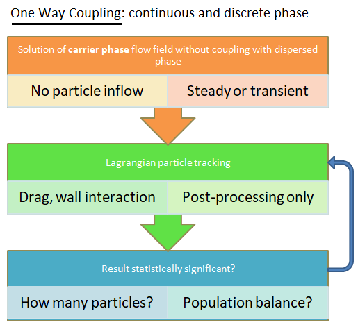
Phase-coupling mechanisms strongly influences the behavior of the continuous and dispersed phase. There are 3 different types of couplings present in particle-laden fluid flows.- One-way coupling or uncoupled approach: fluid → particles - this is appropriate only with very dilute concentration (< 0.01% volume fraction) of particles and has no significant effect on turbulence. The flow field is calculated assuming no presence of particle - fixed continuous phase flow field (that is before the particles is injected into the flow) and tracked as they injected into the flow. The particles does not interact with any other particles during its track throughout the flow domain.
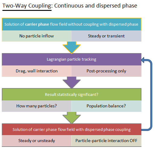
- Two-way coupling: fluid ↔ particles - this coupling becomes important when the volume fraction of particles is in the range 0.01% - 10% and affects both dissipation and production of TKE. The flow of fluid is necessarily solved along with the movement for Lagrangian particles. This is enabled in ANSYS FLUENT by switching on "Interaction with Continuous Phase" option in the Discrete Phase Model dialog box. To control the frequency at which the particles are tracked and the DPM sources are updated, "Number of Continuous Phase Iterations per DPM Iteration" option exists. Option "Update DPM Sources Every Flow Iteration" is available for unsteady simulations.
- Four-way coupling: fluid ↔ particles + particle collisions: the particle - particle interaction becomes important if volume fraction of particles is > 10%. Note that the mass fraction can be still higher due to large difference in the densities of the solid and gas / liquid.
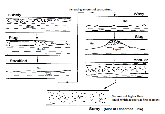
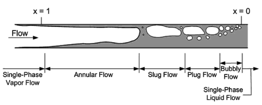
Flow Regimes
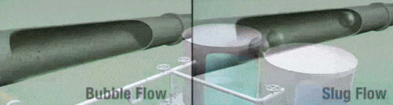
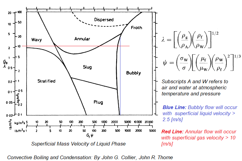
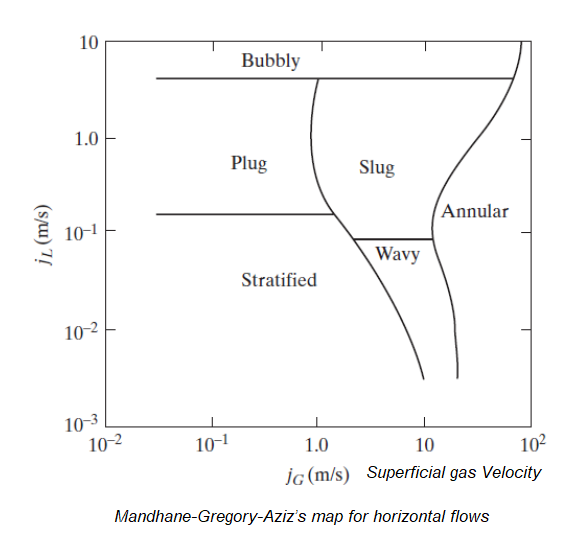
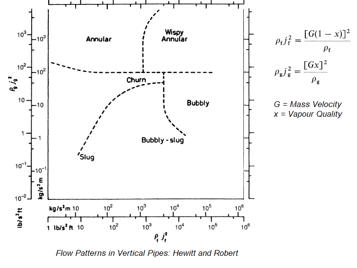
There is no unique and uniform procedure to describe and classify flow patterns in two-phase mixtures. Usually flow pattern maps (such Baker's map, Hoogendoorn map, Mandhane-Gregory-Aziz map, Mukherjee and Brill map, Taitel and Duckler map, Spedding and Nguyen map for horizontal flows, Hewitt and Roberts map, Griffith and Wallis map, Golan and Stenning map for vertical upward flow in a tube) are used to identify the flow regimes. The Taitel and Dukler map was evolved based on tests dealing with condensation with water, methanol, propanol, R113, N-pentane in 24.4 [mm] tube. A flow pattern worth mentioning is "slug flow". Slug literally means 'strike' or 'thump'. In this type of flow, wave of liquids hit the upper section of the pipe with a higher velocity than the average liquid velocity. Thus, pressure fluctuations are a common in such type of flows.Flow Regime: Horizontal Conduits
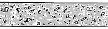
Bubbly Flow: it represents a flow of discrete gaseous or fluid bubbles in a continuous phase. The homogeneous multi-phase models can be used for this flow regime.
Gravity, buoyancy, interfacial tension, pipe diameter, friction and pressure define the shape of a flow. The various spatial shapes the flow takes in two- or three-dimensions are often referred to as flow pattern. There are many types of flow patterns that could exist in two-phase flow depending on a specific set of flow parameters including diameter and/or pipe inclination. The various flow regimes based on fraction of gas phase in horizontal and vertical pipes are described in following pictures.
Mandhane-Gregory-Aziz's map: note the axes are different from the Baker's map
Flow Regime: Vertical Conduits
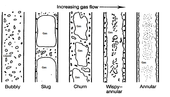
Bubble Regime: In this type of flow regime, there is a distribution of secondary phase bubbles throughout the continuous liquid phase. The bubbles may vary widely in size and shape but they are typically nearly spherical and are much smaller than the diameter of the tube itself. The average bubble size increases with increase in the gas flow rate. The homogeneous multi-phase models can be used for this flow regime.
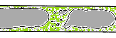
Slug Regime: When the gas flow rate is increased beyond a certain value, many bubbles collide and coalesce to produce slugs of gas or to form larger bubbles known as slug flow. These bubbles are also known as Taylor bubbles. The gas slugs have spherical noses along the direction of flow and occupy almost the entire cross section of the tube, being separated from the wall by a thin liquid film. Between slugs of gas there are slugs of liquid in which there may be small bubbles entrained in the wakes of the gas slugs.
Churn Regime: When the velocity of the flow in increased further, the structure of the flow becomes unstable with fluid travelling up and down in an oscillatory and chaotic type but with a net upward flow. The slug flow pattern is destroyed and over most of the cross section there is a churning motion of irregularly shaped portions of gas and liquid.
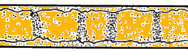
Annular Regime: Further increase in the gas flow rate causes separation of the phases where the liquid flows mainly on the wall of the tube and the gas in the core area. In the annular flow regime the entrained droplets do not coalesce to form larger drops.
Reference: youtube.com/watch?v=pkhVxqDg_fk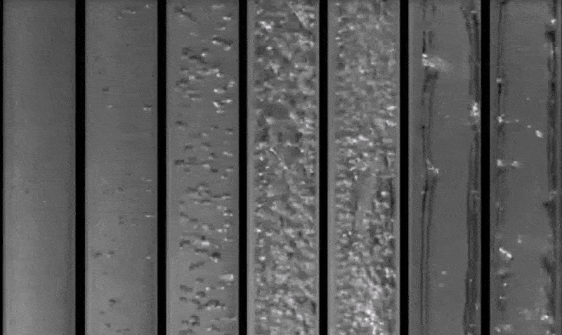
Wispy-Anular Regime: When the liquid flow rate is increased further, the volume fraction of liquid increases in the gas core where the entrained liquid is present as relatively large drops and the liquid film contains gas bubbles. The homogeneous multi-phase models can be used for this flow regime.
Terminologies associated with two-phase (TP) flows are described here.
- Total Mass Flow Rate, mTP [kg/s]: it is defined as the sum of the mass flow rate of the liquid phase mL and the gas phase mG.
- Total Mass Flux, GTP [kg/m2-s]: it is defined as the sum of the mass flux of the liquid phase GL and the gas phase GG.
- Flow Quality, x [%]: Flow quality is defined as the ratio of gas phase mass flow rate to the total mass flow rate, that is x = mG / mTP.
- Superficial Velocity or Volumetric Flux, j, U [m/s]: 'Superficial' velocity is derived based on total cross-section of the pipe even though actual flow may occur only through fractional area of the pipe. Thus, USUP-G = GG / ρG / A and USUP-L = GL / ρL / A
- Slip Ratio, S or σ [%]: It is defined as the ratio of the average 'superficial' velocity of the gas phase to the average 'superficial' velocity of the liquid phase. S = (UG/UL). When the slip ratio = 1, both liquid and vapour (gas) phase move at same speed. This assumption leads to a two phase model known as homogeneous or zero-slip model.
- Void Fraction or Volume Fraction, α [%]: Void fraction is defined as the ratio of the cross-sectional area occupied by the gas to the total cross-sectional area of the pipe. Since this ratio will vary along the length or flow direction, an integral or sum results in a ratio that gives the volume of space the gas phase occupies in two-phase flow in a pipe. Thus, for a homogeneous model:
Void fraction, like the flow is a random and fluctuating quantity. However, it is assumed that the it is a stationary random process such that the simple time average equals ensemble average. Instruments such as gamma ray densitometry, capacitance probe and resistance probes give the distribution of void fraction though results are rarely conclusive and agreement with each measurement method.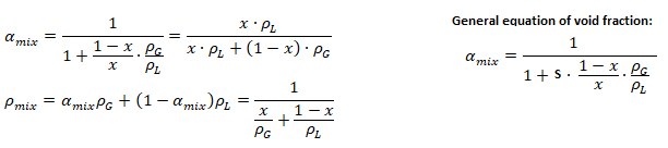
- Volumetric Quality, β [%]: The volumetric quality is the ratio of the volumetric flux of a phase to the total volumetric flux.

- Mass Quality, x [%]: It is the ratio of the mass flux of a phase 'i' to the total mass flux of all the phases. This is also known as "flow quality" or "dryness fraction" in case of liquid-gas mixtures.
β = x.UG / [x.UG + (1 - x). UL), Slip ratio S = (UG/UL) = β/α × [1 - α] / [1 - β].
- Drift Velocity, Ui [m/s]: The drift velocity of a component is defined as the velocity of that phase in a frame of reference moving at a velocity equal to the total volumetric flux.
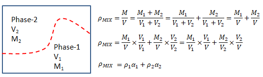
- Mixture Density: ρTP = α × ρG + (1 - α) × ρL where α is the volume fraction.
- Froude Number: A measure of wavinesss of the liquid surface -

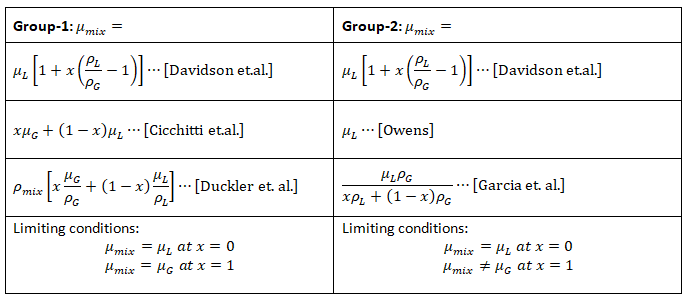
- Mixture Viscosity: There are many definitions of mixture viscosity used by various researched to fit the test data.
Nomenclature as per OpenFOAM
- phi [φ]: generic phase variable, mixture variable in "mixture models"
- alpha [α]: volume fraction of a phase, α = 1 for mixture models
- rhoi [ρi]: density of ith phase
- p_rgh: Modified pressure p* = p - ρg.x obtained by removing hydrostatic pressure component from static pressure P = p/ρ
- Dispersed phase: phase with lower volume fraction
- Carrier phase: phase with higher volume fraction
- Particulate loading: The particulate loading is defined as the mass fraction ratio of the dispersed phase to that of the carrier phase
Separated Flow Model
In separated flow models each phase/fluid is assumed to flow separately from one another. Most separated flow models assume different velocities for each phase unlike homogeneous flow models where both of the fluids are assumed to have the same velocity. A method of using a two-phase frictional pressure drop multiplier 'φ' is a popular method of developing a separated flow model pressure drop correlation. This type of analyses have been found appealing for most researchers because single-phase flow techniques and results are analogically related to two-phase flows by this method. This instance has a benefit of avoiding ambiguity over which physical property of the phases to use, such as which viscosity of either of the phases to use during calculation of two-phase pressure drop.There are two ways of modelling the two-phase friction multiplier.
- The first one is assuming all the flow to be as one out of the two phases present such as all flow as liquid or all flow as gas. The implication here is to use the total mass flux (the sum of the mass fluxes for each phase) instead of the mass flow for each phase. Subscripts 'LO' and GO' indicate liquid only and gas only respectively.
- The second method is to assume as if only one of the phases exist and use the respective mass flux only while calculating the Reynolds number. Therefore in this case, only the respective mass flux is used to calculate the Reynolds number.
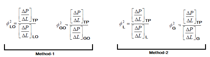
Lockhart and Martinelli also introduced a dimensionless parameter X defined as follows. The two phase friction multiplier φL is a function of X as per the equation shown. The constants as per Chisholm are also tabulated.
The LM-parameter 'X' relates the single phase pressure drop each for liquid and gas phase as if each fluid is flowing alone in the pipe and therefore respective mass fluxes should be used.
| Flow mechanism | Value of C | |
| Liquid | Gas | |
| Viscous (Laminar) | Viscous (Laminar) | 5 |
| Turbulent | Viscous (Laminar) | 10 |
| Viscous (Laminar) | Turbulent | 12 |
| Turbulent | Turbulent | 20 |
- Inputs: mass flow rates of each phase or mass flow rate of one phase and volume fraction of the other phase, pipe diameter, operating mean pressure and temperature
- Calculate the Reynolds number for each phase assuming as if each fluid is flowing alone in the pipe. Output: ReL and ReG. Note that the turbulent flows for two-phase flows in pipe starts at Re = 1000.
- After viscous-turbulent classification for each phase, calculate dimensionless parameter X that is calculate either of [XTT XTV XVT XVV].
Wave Proparation in Two-phase Flows
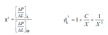
One of the important effect of presence of gas phase (such as air) in water is decrease in speed of sound in the liquid phase. This reduction in speed of sound will cause shock waves to occur at lower fluid velocities.
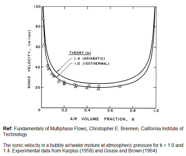
Taitel and Dukler Map: Flow regime calculation procedure
The method uses different coordinates for each transition boundary:- Stratified to annular: X, F
- Stratified to intermittent: X, F
- Intermittent to dispersed bubble: X, T
- Stratified smooth to stratified wavy: X, K
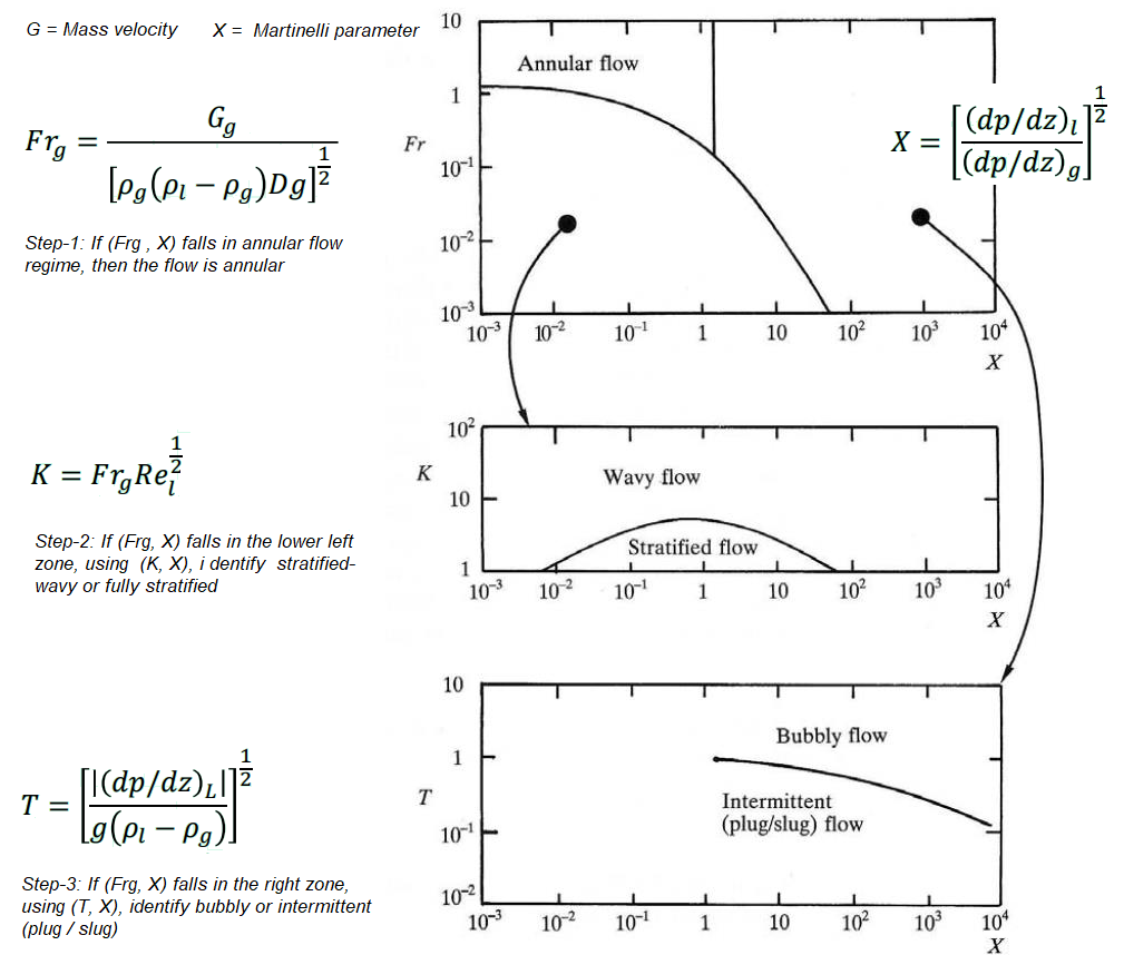
- Cross-section area of tube, A = 0.0491 [m2]
- Mass velocity of mixture, G = 10 [kg/s] / 0.0491 [m2] = 203.7 [kg/m2.s]
- Mass velocity of gas, GG = x.G = 0.20 × 203.7 = 40.7 [kg/m2.s]
- Mass velocity of gas, GL = (1 - x).G = 0.80 × 203.7 = 163.0 [kg/m2.s]
- Reynolds numbers based on superficial velocities: ReG = GG.D/μG = 509,300, ReL = GL.D/μL = 40,744
- Friction factors: fG = 0.079 / ReG0.25 = 0.0030, fL = 0.079 / ReL0.25 = 0.0056
- Calculate pressure gradients: [dp/dz]G = [2fG.GG2]/[ρG.D] = 7.85, [dp/dz]L = [2fL.GL2]/[ρL.D] = 1.18
- Calculate Martinelli Parameter, X = [1.18 / 7.85]0.5 = 0.39
- Calculate Froude number for gas phase, FrG = 0.37
- Locate the point [FrG, X]. It falls in lower-left zone. Hence, step-2 described above applies.
- Calculate parameter K = FrG × ReL0.5 = 74.5
- Locate the point [K, X]. The flow is in wavy regime.
This page summarizes the multi-phase cases supplied with OpenFOAM.
Some of the resource from the web are listed below. IPR: the ownership and copyright of these documents lie with the author mentioned in the document.- This web page from CHALMERS university is a comprehensive list of article, research report and presentations on OpenFOAM
- This is a wiki page which is an excellent attempt to categorize the documents with ease of search.
- Since this page is intended for multiphase phenomena only, some of the PDF files I read and used to get insight into the available utilities in OpenFOAM are linked below. Note that the documents are still owned by respective authors and is produced here for reference only.
Thus, if both or all the phases are to be modelled as continuous phases, Eulerian approach is used. When a discrete phase (spatially not continuous) is to be modeled, a Lagrangian frame of reference is used in which spherical particles of pre-defined size distribution is dispersed in the continuous phase (the spherical particles may represent parcels of droplets or bubbles). The fluid phase is modeled as a continuum where time-averaged Navier-Stokes equations are solved to get flow field while the discrete phase is solved by tracking a large number of particles (parcels, bubbles, or droplets) through this calculated flow field. Thus, a Lagrangain approach includes and requires:
- calculation of discrete phase trajectory for both steady and unsteady flows
- estimation of effects of turbulence on dispersion of particles due to vortices and eddies present in the continuous phase
- account for heating or cooling of the discrete phase including break-up of droplets in sprays, vaporization and boiling of such droplets
- the volume fraction of discrete phase should be < 10% even though mass fraction can be higher due to higher density of solids as compared to liquids. Thus, this method will not be appropriate for fluidized bed where volume fraction of discrete phase is > 50%. Note that twoPhaseEulerFoam should be used in such applications. The Euler-Lagrangian solver coalChemistryFoam is not related to fluidized beds.
CSTR, Emulsification
- Vigorous stirring or agitating two or more immiscible liquids results in the dispersion of one phase in the other in the form of small droplets whose size and shape depend on the equipment, the material properties such as density and surface tension and the operating conditions.
- The mixing of two immiscible liquids is called emulsification where a binding agent called emulsifier holds the two phase together and dispersed. Icecream, milk, mayonnaise, sauces are some of the examples of emulsion.
- Prediction of drop size distributions in turbulent liquid-liquid dispersions in static mixers thus becomes one of the most important output of any test set-up or numerical simulation methods.
- Similarly, any phenomena dealing with droplets require a mathematical model to capture break-up, aggregation and coalesce phenomena of the droplets. One such approach is Population Balance Equations (PBE) - particle size distribution by means of a transport equation, similar to k and ε equations.
- Since each phase is a continuum, Euler-Euler multiphase models are used to simulation emulsification process.
DPMFoam: Discrete Phase Model - This is another multi-phase solver which includes the effect of the discrete phase particulate volume fraction on the continuous phase. This utility is recommended for dense particle flow simulation. Though there is no strict and standard definition of 'dense' particle-laden flow, a volume fraction of 10% or higher is usually considered 'dense'. The solver uses existing functionality for particle clouds and their collisions, which directly resolves particle-particle interactions. Official description is "Transient solver for the coupled transport of a single kinematic particle cloud including the effect of the volume fraction of particles on the continuous phase".
The particle size (diameter) distribution is an integral part of DPM simulation, both in OpenFOAM or commercial programs like Siemens STAR-CCM+ or ANSYS FLUENT. In Rosin-Rammler distribution, the continuous diameter distribution is divided into a number of discrete intervals. The underlying assumption for the Rosin-Rammler distribution is that the mass fraction of particles having a diameter > d is an exponential function of the particle diameter d. Thus: β(d) = 1 / exp(d / dM)n where dM = mean diameter and n = spread parameter. The steps required to calculate mean diameter and spread parameter are as follows:- Divide the minimum and maximum diameter into discrete intervals: d0, d1, d2 ...dN. But how will one know minimum and maximum diameters a-priori? It is an iterative process and one need not know all information well in advance.
- From sieve analysis, estimate the mass fractions of particles below di where i = 1, 2, 3 ...N.
- Plot the graph: MF(d) vs. d(i).
- Plot a horizontal line which crosses vertical axis at 1/e = 0.3679
- The intersection of these two lines is the mean diameter, dM.
- For each discrete interval, calculate spread parameter ni = ln[0 - ln(MF[di])] / [ln(di) - ln(dM)] i = 1, 2, 3 ...N.
- Calculate the average of ni, which is the spread parameter to be input in most of the CFD simulation software such as ANSYS FLUENT.
- Reports>Discrete Phase>Sample>Set Up
- Pick appropriate boundary say "inlet" or "outlet", injection setting, then "Compute". Make sure that the chosen boundaries represents all particles that flow into the system or flow out of the system.
- This action will write to disk a file called "inlet.dpm" or "outlet.dpm" depending upon the boundary selected which will record the profile of particles at that boundary.
- To plot histogram, use GUI option: Reports > Discrete Phase > Histogram > Set Up. Select "Read" then pick the file just saved (*.dpm). Select appropriate entry under "Sample", "Variable" and "Weight" tabs. Select "Plot".
Particle-Wall Interactions:
Another aspect of a DPM simulation is modelling of "particle-wall interaction". The particle may either reflect after hitting the wall or get captured by the wall (stick to it). To check whether particle - wall collisions is likely to occur or not, the Stokes number gives an indication whether the particles will follow the flow or hit the wall.
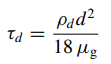
The Stokes number is defined as the ratio of particle response time (a measure of how fast the particles react to a change in fluid velocity) to a characteristic timescale of the flow (how fast changes in flow occur). The particle relaxation time is a measure of its inertia and denotes the time scale with which any slip velocity between the particles and the fluid is reduced to zero. The relaxation time (τd) is usually the time required by the particle to respond to changes in fluid velocity and depends on particle size (d), particle density (ρd) and fluid viscosity (μg).
For water (density = 998.2 [kg/m3]) droplets in air (viscosity = 18.0E-6 [Pa.s]), the relaxation time as function of particle diameters are tabulated below.
| d | τd | ||
| [mm] | [μm] | [s] | [ms] |
| 1.00E-02 | 10.00 | 3.08E-03 | 3.08E+00 |
| 4.00E-03 | 4.000 | 4.93E-04 | 4.93E-01 |
| 1.60E-03 | 1.600 | 7.89E-05 | 7.89E-02 |
| 6.40E-04 | 0.640 | 1.26E-05 | 1.26E-02 |
| 2.56E-04 | 0.256 | 2.02E-06 | 2.02E-03 |
| 1.02E-04 | 0.102 | 3.23E-07 | 3.23E-04 |
| 4.10E-05 | 0.041 | 5.17E-08 | 5.17E-05 |
The characteristic time scale of the fluid is often taken as the time constant for turbulence defined as the ratio between turbulent kinetic energy (k) and turbulent dissipation rate (ε).
- If the particle response time is << fluid timescale, the Stokes number is << 1, the particles will react instantly to any change in the fluid velocity and hence follow the flow closely.
- If the particle response time is >> the fluid timescale, the Stokes number is >> 1, the particles will be unaffected by changes in the flow.
- In normal collisions (in oblique collisions, respective orthogonal components can be used), the co-efficient of restitution is defined as the ratio of the particle rebound velocity to the particle incidence velocity. As the particle normal velocity decreases, the particle rebound velocity decreases proportionately and eventually reaches a point where no rebound will occur resulting in particle getting trapped by the wall. This maximum velocity below which particles are trapped is known as the capture or critical velocity.
Particle-Particles Interactions:
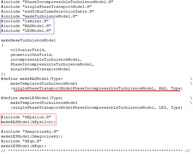
In ANSYS FLUENT, particle-particle interactions is included in Discrete Element Model using Discrete Element Method Collision Model. The implementation is based on the work of Cundall and Strack and accounts for the forces that result from the collision of particles designated as "soft sphere" approach). The forces from the particle collisions are determined by the deformation, which is measured as the overlap between pairs of spheres or between a sphere and a boundary. The collision forces available are (a)spring, (b)spring-dashpot and (c)friction. However, the details of the flow around the particles (e.g. vortex shedding, flow separation, boundary layers) are neglected.The term 'cloud' in OpenFOAM represents the overall presence of all particles, whether they're active or not. Since, this is a transient solver, it is based on PIMPLE algorithm. Turbulence models available in this utility are [a] laminar, [b] k-ε RANS and [c] LES as shown in the header file of the source code.
Relaxation Time of Particles
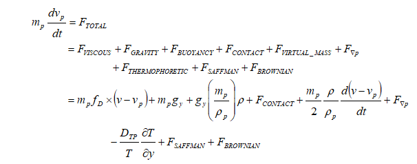
When a particle experiences change in velocity (that is acceleration), it may not immediately get accelerated to the fluid velocity as stated in Newton's first law of motion. The time scale with which any slip velocity between the particles and the fluid is equilibrated is called particle relaxation or response time and it is a measure of particle inertia. In other words, relaxation time is the time required by the particle to respond to changes in fluid velocity and depends on particle size (dp, density ρp and fluid viscosity μ. The relaxation time is calculated as τ = [ρp dp 2] / [18μ]Forces acting on particles
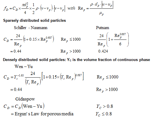
Net force = drag force + added mass effect + history effect + gravitational force + Buoyancy force + Lift force + Intercollision force + Brownian force + Thermophoresis force + Magnus force + Basset Force. The drag force is the most dominant force for particle motion, especially when the particle Re ≤ 100.- Gravity - the well-known force present everywhere!
- Buoyancy - force due to density difference of the particle and continuous phase.
- Pressure gradient - the force due to pressure difference along the direction of motion of the particle.
- Intertia: The acceleration or deceleration of the particle in a fluid requires also an accelerating or decelerating of a fluid surrounding the particle (important for liquid-particle flows).
- Added mass (ma ): The term refers to the additional force (FA) required to accelerate the solid body through a fluid. As the body and the fluid cannot occupy the same volume simultaneously, a force is required to displace the fluid. Though this force can be neglected in gas flow, the force can be significant in liquids due to the high density of liquids. By definition, the added mass force is in phase with the acceleration 'a' (no time lag) which can be expressed in terms of a virtual mass. This will lead to Newton’s 2nd law expressed as FA = (mP + mA) × a.
- Slip-shear lift force: particles moving in a shear layer experience a transverse lift force due to the nonuniform relative velocity over the particle and the resulting non-uniform pressure distribution. Saffman's lift force is caused by the shear of the surrounding fluid which results in a non-uniform pressure distribution around the particle. This force assumes significant magnitudes only in the viscous sublayer where shear rate is the highest. If a particle leads the fluid motion, then the lift force is negative and the particle moves down the velocity gradient towards the wall. Conversely, if the particle lags the fluid, then the lift force is positive and it moves up the velocity gradient away from the wall.
- Slip-rotation lift force: particles, which are freely rotating in a flow, may also experience a lift force due to their rotation (Magnus force).
- Thermophoretic force: a thermal force moves fine particles in the direction of negative temperature gradients (important for gas-particle flows). Brownian and Thermophoretic forces are important for sub-micron particles. Brownian force is caused by the random impact of particles with agitated gas molecules. Thermophoretic force is caused by the unequal momentum exchange between the particle and the fluid where higher molecular velocities on one side of the particle due to the higher temperature give rise to more momentum exchange and a resulting force in the direction of decreasing temperature.
- The force required to maintain the flow pattern was approximated by Basset and depends on the history of the particle trajectory and hence is called the "history effect". Basset forces is negligible for particles with density substantially larger than the fluid density.
- The solidParticleCloud class in OpenFOAM is a class that calculates the movement of particles. In ANSYS FLUENT, time integration of the particle trajectory
equations described below is controlled by following two parameters:
- Maximum number of time steps: maximum number of time steps (default = 500) used to compute a single particle trajectory via integration of particle Force Balance Equation, it is used to abort trajectory calculations when the particle never exits the flow domain with trajectory fate reported as 'incomplete'. Simulation where trajectories are reported as incomplete within the domain and the particles are not recirculating indefinitely, one need to increase the maximum number of steps (up to a limit of 109) to get more trajectories.
- Length scale/step length factor: set the time step for integration within each control volume, it is ∝ to the integration time step and is equivalent to the distance that the particle will travel before its motion equations are solved again and its trajectory is updated. A smaller value for the Length Scale increases the accuracy of the trajectory.
- Rarefaction Effect: Rarefaction effect is governed by Knudsen number which is defined as the ratio of the mean free path of the gas molecules to the particle size. This effect is important for sub-micron particles (< 1 μm) for non-continuum regime, where continuum regime is defined as Kn ≤ 0.1; transition regime 0.1 < Kn Lt; 10 and free-molecule regime as Kn ≥ 10.
Lagrangian >> sprayFoam - To predict the behavior of a spray such as atomizer, the discrete phase model is used which includes a secondary model for breakup. Due to constraints on mesh resolutions, spray models are not entirely predictive. Accurate submodels is needed for detailed spray processes such as atomization, drop drag, drop-turbulence interaction, vaporization, drop breakup, collision and coalescence and spray/wall interaction. The Lagrangian Discrete Phase Model (DPM) is the work-horse approach in commercial codes for simulating spray modelling. In OpenFOAM, the utility is named as sprayFoam (folder lagrangian/ sprayFoam / aachenBomb) - earlier known as dieselFoam. case /constant /injectorProperties file contains spray (injection) information). E.g. injector is located at 100 [mm] on y-axis and injects in the negative y-direction. X is the mass fraction of a specific specie. The massFlowRateProfile specifies how the mass flow rate should vary wither time. From time t0 → t1, the mass flow rate is m0. This is done to simulate opening and closing of the injector. The left column of the massFlowRateProfile is ti and the right, mi. The tutorial in PDF format can be found here. A tutorial on description of particle injection in OpenFOAM can be found here.
injectorType unitInjector;
unitInjectorProps  {
  position    (0  0.1  0);
  direction   (0 -1.0  0);
  diameter    0.0002;
  Cd          0.9;
  mass        6.0e-06;
  temperature 320;
  nParcels    5000;
  X (
    1.0
  );
massFlowRateProfile (
  (0.00    0.125)
  (4.0e-05 6.375)
  (8.0e-05 8.500)
  ...
);
Atomization: Kelvin-Helmholtz Jet Breakup Model. Drop breakup regimes are:
- First breakup stage: Deformation and flattening occurs in the range Weber number We ≤ 12.
- Second breakup stage: Bag breakup, Shear breakup, Stretching and thinning breakup, Catastrophic breakup.
- Bag breakup: 12 ≤ We ≤ 100
- Shear breakup: We < 80
- Stretching and thinning breakup: 100 ≤ We ≤ 350
- Catastrophic breakup: We > 350
MPPICFoam (MultiPhase Particle-In-Cell method): This is a "Lagrangian solver" having LPT (Lagrangian Particle Tracking) capabilities and can be used for modelling particles in continuum. This method simulates solid phase as parcels and is used to represent collisions without resolving particle-particle interactions. This solver is identical to DPMFoam, but without the collisions between particles.. Quote from a post by Bruno Santos on cfd-online.com: ||The solvers DPMFoam and MPPICFoam are virtually identical, except that the first one uses "basicKinematicCollidingCloud" as the base cloud type and the second one uses "basicKinematicMPPICCloud"||
The particles are assumed to be rigid, spherical and are thus described by diameter, density, coefficient of restitution (rebound properties) and coefficient of friction (tangential drag during collision). Hence, collisions between particles are modeled using keywords identifying properties of spring, friction slider and dash-pot in appropriate dictionaries.
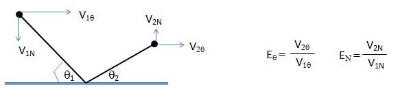
There are two time-steps involved: fluid flow time steps (the time-steps used for solution of continuous or carrier phase) and particle tracking time steps which decides the time step for particle injection. In ANSYS FLUENT one can perform steady state trajectory simulations even when selecting a transient solver for continuous phase equations or specify transient particle tracking when solving the steady continuous phase equations. This is explained in following diagram. ![]()
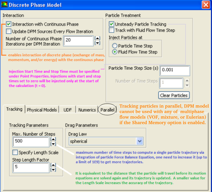
Number of Particle Streams: This option controls the number of droplet parcels that are introduced into the domain at every time step.
Note the options at top right quadrant: Inject particles at (i)Particle Time Step and (ii)Fluid Flow Time Step. The option (i) requires two entries (a)Particle Time Step Size in [s] and (b) Number of Time Steps. Option (ii) requires only (a) Particle Time Step Size. To start the particle injection at t = 0, set "Start Time" of inject = 0. In order to keep the particle injection long after the time period of interest, set a large value for the Stop Time, for example 500 [s] which ensures that the injection will essentially never stop.Turbulent Particulate Dispersion
One of the salient features of turbulent flows is their higher diffusivity species, momentum and energy to mix and transport much faster than is done by molecular diffusion. Turbulent dispersion is best studied from a Lagrangian viewpoint by following the motion of fluid elements. There are two methods, deterministic or Stochastic model to acount for the turbulent dispersion. Deterministic models take into account the slip velocity and calculate the interface mass/heat transport rates using the slip velocity by taking into account the Reynolds number and the Sherwood/Nusselt number. Stochastic models are similar to the deterministic models but they also take into account the effect of turbulent fluctuations on particle motion and interface transport.In ANSYS FLUENT, the particle dispersion in the turbulent flow field is accounted for by following two methods:
- Stochastic tracking/Discrete Random Walk (DRW) model: known as the "Eddy Interaction Model", each injection is tracked repeatedly to obtain a statistically meaningful sampling. The "number of tries" option in the 'Injections' panel = the number of times every injection needs to be tracked. Mass flow rates and exchange source terms for each injection are divided equally among the multiple stochastic tracks. Without Stochastic Tracking, only one particle trajectory is calculated for each injection point and the effects of turbulence are ignored which many not be a valid assumption. For 'N' number of stochastic tries, 'N' values of perturbation are calculated for 'N' different regions in the probability distribution function (PDF) and 'N' different particle tracks are generated from the same injection point. But the mass flow rate for the injection at that point will be divided equally among the 'N' particles, thus matching the total mass flow rate through the inlet while accounting for the particle dispersion. This accounts for the dispersion effect and ensures the calculations are performed for 'N' different trajectories instead of just one particle track. One drawback of the EIM/DRW model is that it does not account for the strong anisotropic nature of turbulence inside the boundary layer as it is based on an assumption of isotropic turbulence.
- Particle cloud approach: The particle cloud model considers the statistical evolution of a particle cloud about a mean trajectory. A "particle cloud" is required for each "particle type" in this model. The concentration of particles about the mean trajectory is represented by a Gaussian probability density function (PDF) whose variance is based on the degree of particle dispersion due to turbulent fluctuations. The mean trajectory is obtained by solving the ensemble-averaged equations of motion for all particles represented by the cloud. The cloud enters the domain either as a point source or with an initial diameter. The cloud expands due to turbulent dispersion as it is transported through the domain until it exits. The value of the PDF represents the probability of finding particles represented by that cloud with residence time t at location xi in the flow field. This model is computationally less expensive but is less accurate.
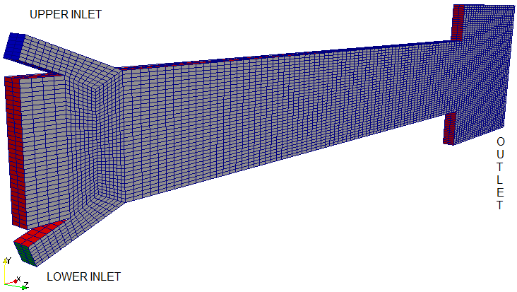
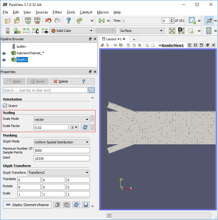
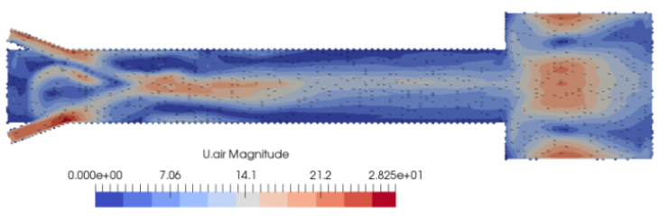
Lagrangian >> MPPICFoam >> injectionChannel - The computational geometry and animation of particle tracks in a mixing phenomena of two streams of particle-laden gas is described below.
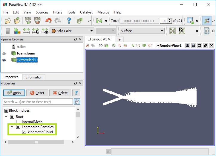
Particle tracking in ParaView
To show particles in ParaView from a kinematicParcleFoam simulation, choose "kinematicCloud-lagrangian" instead of internalMesh in the Mesh Parts. For particle tracking in ParaView, [a] either the utility particleTracks can be used or [b] convert the case to VTK format using foamToVTK utility. Copy the particleTrackProperties dictionary into the constant directory and execute the utility: particleTracks. This will generate necessary files to visualize the particle trajectories in ParaView. The location of the file particleTrackProperties is:$FOAM_UTILITIES/postProcessing/lagrangian/particleTracks/particleTrackProperties
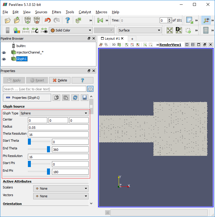
Both the particleTracks and foamToVTK utility will create a folder named VTK in the case directory which will have further sub-level folders. The folder VTK/lagrangian/kinematicCloud will contain a file kinematicCloud_TTT.vtk files where TTT is the time step. For particle tracking visualization, one needs to open this file. Then, to display the particles the user must filter the Lagrangian field with the Glyph filter, subsequently the scalar option should be selected in the scale mode window along with the spheres as glyphs where Gyph type options [Sphere, arrow, cone, box...] are available.
Glyph settings to plot particles as sphere is shown below 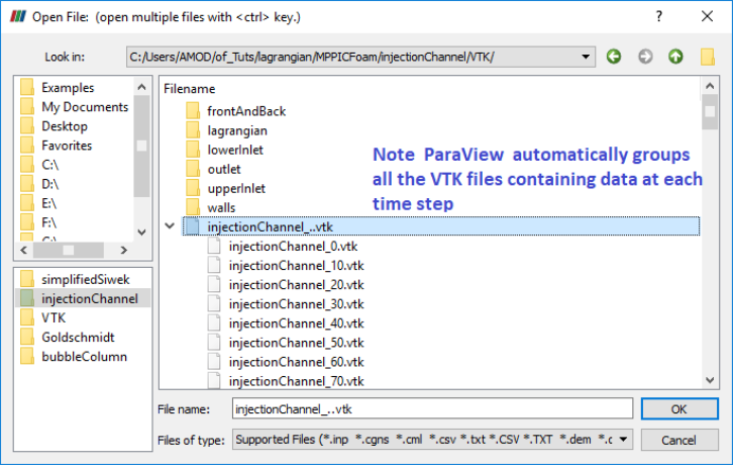
Lagrangian >> simpleReactingParcelFoam >> verticalChannel : a steady state Lagrangian - Eulerian solver for chemical reaction, combustion and particle clouds.
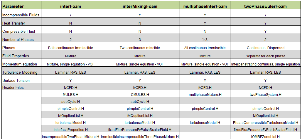
interFoam utility for Multi-phase Flows
Two-phase flows are often broadly categorised by the physical states of the constituent components and by the topology of the interfaces. Thus, a two-phase flow can be classified as gas-solid, gas-liquid, solid-liquid and liquid-liquid in the case of two immiscible liquids . Similarly, a flow can be broadly classified topologically as separated, dispersed or transitional.
interFoam
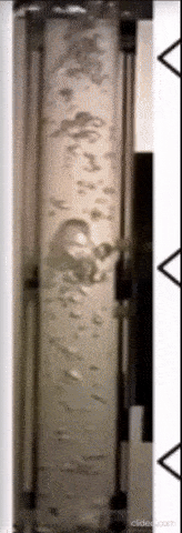
Description as per source code interFoam.c: Solver for 2 incompressible, isothermal immiscible fluids using a VOF (volume of fluid) phase-fraction based interface capturing approach. The momentum and other fluid properties are of the "mixture" and a single momentum equation is solved. Turbulence modelling is generic, i.e. laminar, RAS or LES may be selected. For two-fluid approach see twoPhaseEulerFoam. interFoam has limitations in prediction of sharp interfaces, highly self-aerated flows and air-entrainment phenomena.The following video is an attempt to model air entrainment using multiphase flow. In the left video, you may notice how spherical bubbles are formed due air entrained by water stream entering into the bottle. The interface of the air bubble and water is sharp. This feature is not as prominent in the simulation primarily due to coarse mesh. Capturing a sharp interface between gas and liquid will require a very fine mesh. Some improvements planned are:
- Make the domain shape and size identical: as of now they are in 2:1 ratio to keep the number of mesh counts low.
- Match the boundary conditions such as velocity and its profile at inlet, turbulence parameters at inlet.
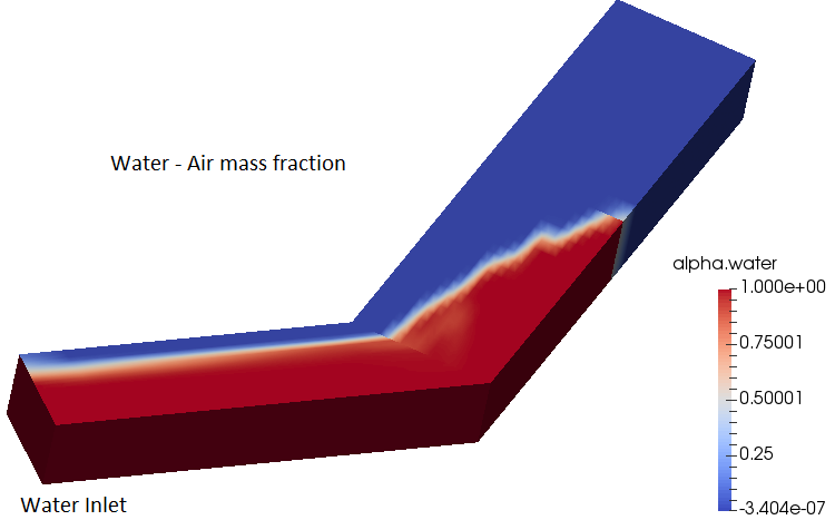
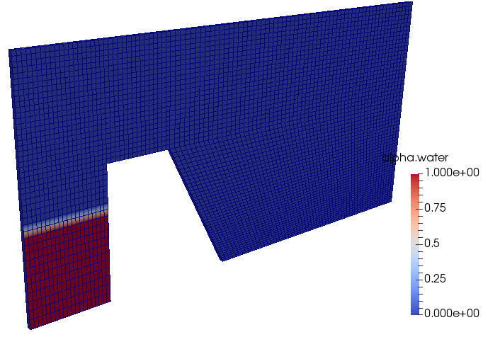
multiPhase >> interFoam >> ras >> angledDuct - Flow of water in an empty angled duct: immiscible two phase flow - there are 3 three implementation with LAMINAR, LES and RAS turbulence as tutorial cases. One of the tutorial with RAS implementation is shown below where water enters into the inlet and fills the duct as it moves towards the outlet.
multiPhase >> interFoam >> ras >> weirOverflow - Over-flow a Weir: 2D - immiscible two phase flow
Volume fraction at t = 0:
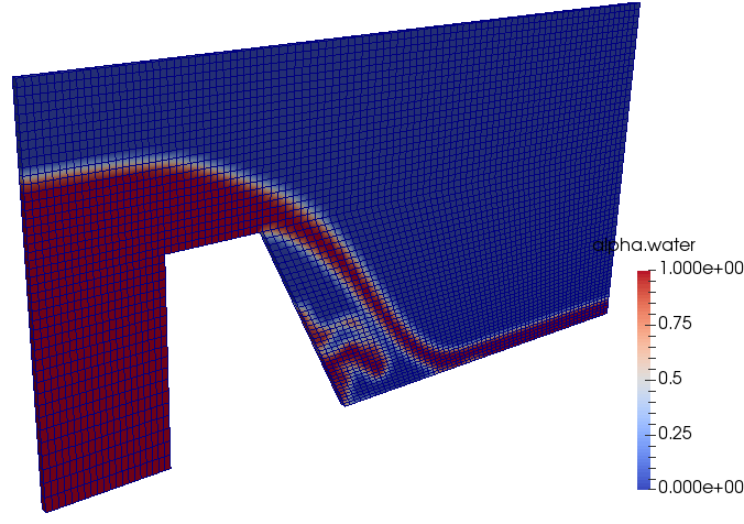
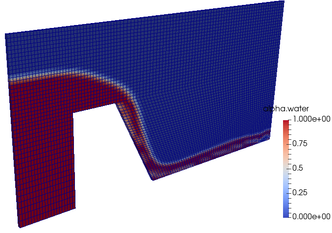
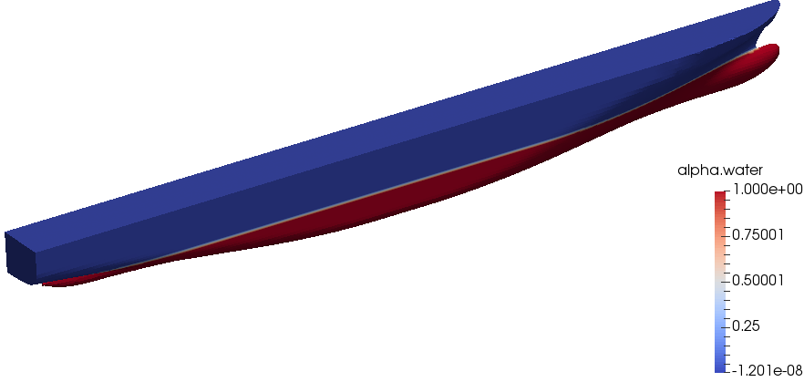
multiPhase >> interFoam >> ras >> DTCHull - Flow over a ship
Geometry and boundary condition: 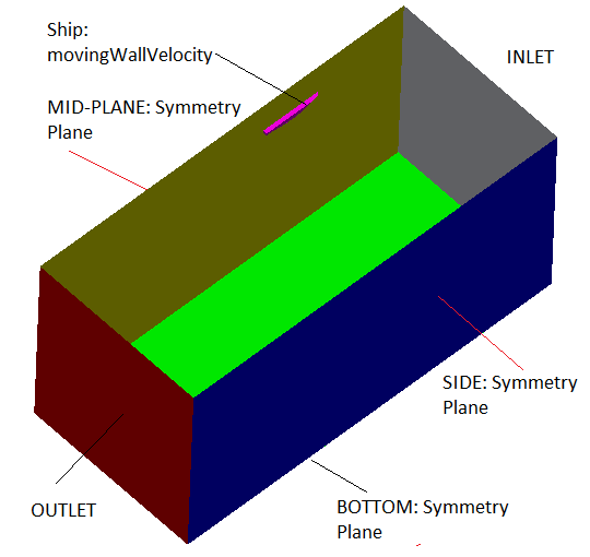
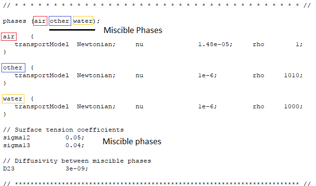
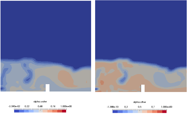
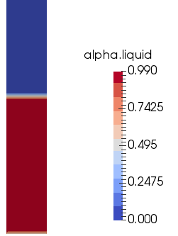
multiPhase >> interMixingFoam >> laminar >> damBreak interMixingFoam - "Solver for 3 incompressible fluids, two of which are miscible, using a VOF method to capture the interface." As per the source code, PIMPLE method is used for pressure-velocity coupling. The settings of tutorial with official version is as follows:
Geometry and Volume fraction of water at t = 0:
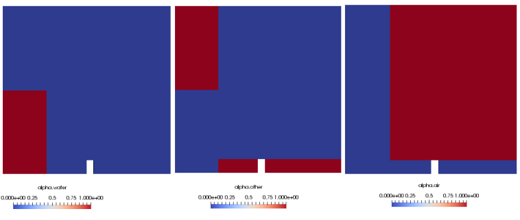
Specification of miscible and immiscible phases:
Volume fraction of miscible phases after 2 [s]:
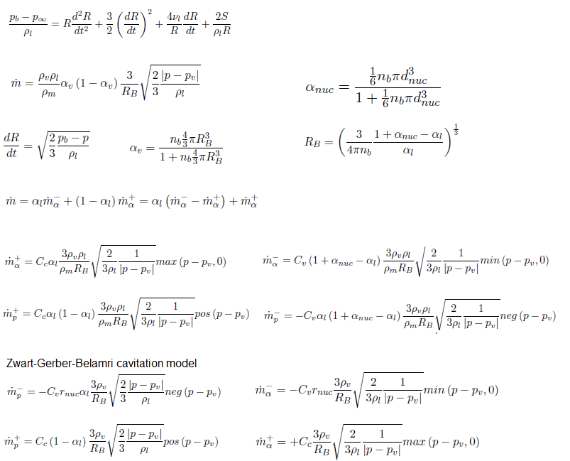
cavitatingFoam
Cavitation refers to the formation of vapor bubbles by local boiling in regions of low pressure within the flow field of a liquid. In some respects, cavitation is similar to boiling, except that the later is generally considered to occur as a result of an increase in temperature rather than a decrease of pressure. Some of the differences between "vapour formation due to cavitation" and that due to boiling are as follows:- It is not possible to raise the temperature of a liquid uniformly where as uniform change in pressure in a liquid can be easily achieved just by controlling the flow passage.
- Cavitation always results in self-destruction downstream the flow, causing large pressure fluctuations. Though vapour formation are also self-destructing as the vapour bubbles move away from the cause, "the surface heat source".
- Bubble formation involves knowledge of Heat Transfer and boundary layer behaviour of the liquid. understanding the Cavitation phenomena does not need any such information.
- Cavitation is almost always detrimental to the surfaces where bubbles collapse. Bubble generation and extinction phenomena in boiling is not so detrimental to the enclosing surfaces.
- Typical location of cavitation is low-pressure (suction side) of the centrifugal pumps. A pump is said to get incipient cavitation if the pressure head generated by the pump reduces by 10% of a "non-cavitating" performance.
Cavitation modeling in ANSYS FLUNET
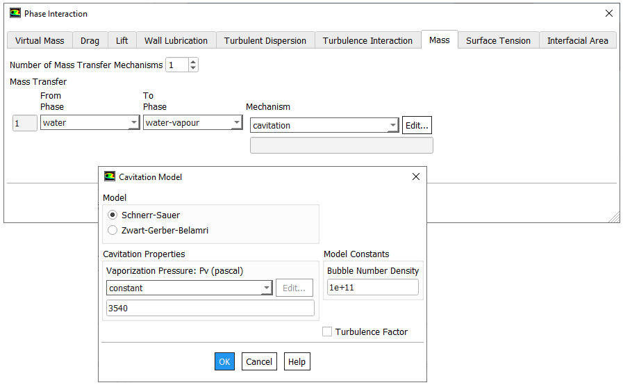
- Solves for two isothermal, incompressible fluids using a Volume of Fluids (VoF) approach where momentum equations are only solved for the mixture.
- Mass transfer through cavitation with the models Merkle, Kunz and Schnerr-Sauer.
- Solves for the liquid fractiona and includes effect of gravity.
- interPhaseChangeFoam uses alphaEqnSubCycle to correct the phase interfaces.
- alphaEqnSubCycle (and alphaEqn) includes vDotAlphal which is part of the phaseChangeTwoPhaseMixtures library.
- vDotAlphal includes mDotAlphal which is different for every cavitation model
- Member functions: rRb, alphaNuc, pCoeff, mDotAlphal, mDotP - as described in the Rayleigh-Plesset and Schnerr-Sauer model equations above.
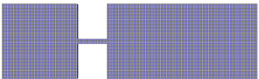
Basic Mesh: Level-0
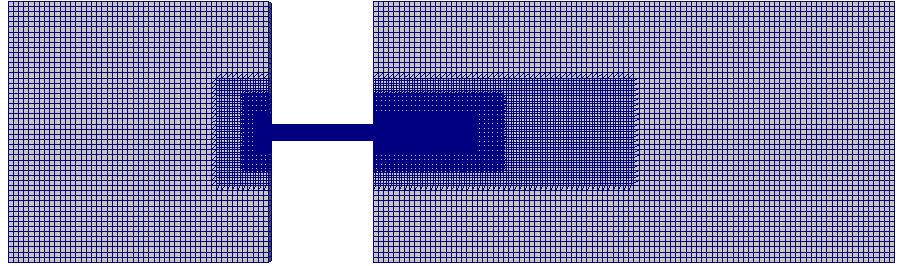
Mesh with level-3 refinement near throat
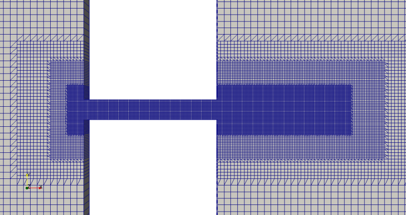
Close-up view of final mesh near throat
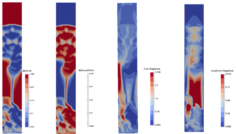
twoPhaseEulerFoam:
This is an Eulerian-Eulerian solver for two (including compressible) fluid phases where one phase is continuous say water and the other phase is dispersed say gas bubbles or solid particles. It may or may not involve heat transfer. Fluidised bed simulations can be performed using this solver. Note that the flow of solids (the particle bed is bubbling) is being modelled here though it is gas assisted and not the granular flow of solid by its own weight.
For two phase flows involving fluids, the thermophysicalProperties are specified by adding suffix after the dictionary 'thermophysicalProperties' such as thermophysicalProperties.air, thermophysicalProperties.water. Special variables for this solver and few settings are described below.- Theta.particles: Granular temperature of solids phase
- alpha.air: Volume fraction of air (fluid) phase
- alpha.particles: Volume fraction of solid phase
- Note that there is a minimum inlet velocity required to ensure fluidization - that is to move the fluid particles from the bed. Hence, chosen inlet velocity should be higher than or equal to minimum fluidization velocity.
- Gravity should be active.
multiphaseEulerFoam:
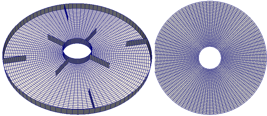
Three or more phases, interface capturing capabilities configured to work with LES and not RANS. Phases can be segregated or dispersed. As per source code: "Solver for a system of many compressible fluid phases including heat-transfer". The application to 2D geometry of a mixing vessel is shown below. This is based on Multiple Reference Frame (MRF) method for sliding interfaces - set by dictionary constant/MRFProperties.
 In case of twoPhaseEurlerFoam, the properties of phases and phase-interactions such as drag, surface tension and interphase mass transfer are specified through the dictionary 'phaseProperties' under 'constant' folder.
kineticTheoryProperties: in older versions of OpenFOAM particle-particle interactions were specified by this dictionary. In recent versions (V6), it is specified using dictionary turbulenceProperties.<phaseName> such as turbulenceProperties.particles where 'particles' is the name of the phase defined in dictionary 'phaseProperties'.
The effective stresses in the solid phase resulting from the particle interaction (collisions) can be described using gas kinetic theory. If equilibrium is on then the algebraic equation for granular temperature is solved instead of the balance equation. This approach is valid when the volume fraction of the solid phase is high (> 10%) and the velocity of the solid phase stays relatively low. The coefficient of restitution is denoted by 'e'. The frictional stresses must be considered in the solid phase stress when the solids volume fraction is high. The 'alphaMax' variable represents the maximum packing limit of the discrete phase. The 'alphaMinFriction' is the value of solid volume fraction when the frictional stresses become important. Fr, eta and p are the material dependent constants used for the calculation of normal frictional stress. The frictional shear viscosity is related to the frictional normal stress by the linear law (Coulomb law) given as μFRIC = PFN sin(φ) where PFN is the frictional normal stress and φ is the angle of internal friction of the particle.
The contents inside turbulenceProperties.particles as per tutorial case multiphase\ twoPhaseEulerFoam\ RAS\fluidisedBed\ is as follows.simulationType RAS;
RAS {
RASModel kineticTheory;
turbulence on;
printCoeffs on;
kineticTheoryCoeffs {
equilibrium off;
e 0.8;
alphaMax 0.62;
alphaMinFriction 0.5;
residualAlpha 1e-4;
viscosityModel Gidaspow; //Syamlal
conductivityModel Gidaspow; //HrenyaSinclair
granularPressureModel Lun;
frictionalStressModel JohnsonJackson;
radialModel SinclairJackson; //Gidaspow
JohnsonJacksonCoeffs {
Fr 0.05;
eta 2;
p 5;
phi 28.5;
alphaDeltaMin 0.05;
}
HrenyaSinclairCoeffs {
L 5.0e-4 ;
}
}
phasePressureCoeffs {
preAlphaExp 500;
expMax 1000;
alphaMax 0.62;
g0 1000;
}
}
The particle-particle interaction force can be activated by setting a value g0 > 0. When the packing limiter is set to on then the solid volume fraction is checked in every cell and then limits the solids volume fraction to alphaMax, the packing limit value.
reactingTwoPhaseEulerFoam / reactingMultiphaseEulerFoam: The simulation of this categories require following 5 files in 'constant' folder -
- chemistryProperties - required to include chemical reactions when 'chemistry' is switched on (for example refer to tutorial case reactingTwoPhaseEulerFoam >> RAS >> bubbleColumnEvaporatingReacting),
- environmentalProperties - specifies gravity,
- combustionProperties - to activate combustion models such as PaSR / XiFoam,
- thermophysicalProperties - specifies type of mixtures and its properties, gas phase reaction scheme, presence of inert species,
- phaseProperties - this dictionary file is specific to this solver and is used to describe interaction between the phases,
- MRFProperties - in case geometry is dealing with rotating domains such as mixer vessel.
compressibleInterFoam
This utility deals with multi-phase flow simulation where phases need to be considered compressible. The suffix 'interFoam' suggest that it is based on Volume-Of-Fluid (VOF) approach. The tutorial case multiphase >> compressibleInterFoam >> laminar >> depthCharge2D deals with a large high-temperature (578 [K]) and pressureized (10 [bar]) air bubble trapped under a water column in a closed cavity. This can be considered a simplified version of high intensity detonation inside water. The computational domain is shown below.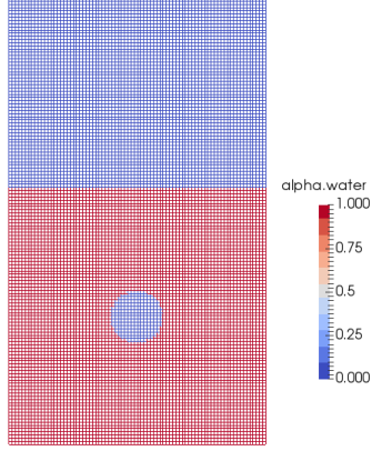
How to convert laminar case to a turbulent case
Change are required in constant/turbulenceProperties file, 0/ directory, system/fvScheme and system/fvSolution files.
| LAMINAR | RANS |
| constant/turbulenceProperties file | |
| simulationType laminar; | simulationType RAS; RAS { RASModel kEpsilon; turbulence on; printCoeffs on; } |
| 0/ folder | |
| * | Add following file and modify boundary names: epsilon k alphat nut nuTilda |
| system/fvScheme | |
| divSchemes { div(phi,alpha) Gauss vanLeer; div(phirb,alpha) Gauss linear; div(rhoPhi,U) Gauss upwind; div(rhoPhi,T) Gauss upwind; div(rhoPhi,K) Gauss upwind; div(phi,p) Gauss upwind; div(((rho*nuEff)*dev2(T(grad(U))))) Gauss linear; } |
divSchemes { div(phi,alpha) Gauss vanLeer; div(phirb,alpha) Gauss linear; div(rhoPhi,U) Gauss upwind; div(rhoPhi,T) Gauss upwind; div(rhoPhi,K) Gauss upwind; div(phi,p) Gauss upwind; div(rhoPhi,k) Gauss upwind; div(rhoPhi,epsilon) Gauss upwind; div(((rho*nuEff)*dev2(T(grad(U))))) Gauss linear; } |
| system/fvSolution | |
| "(T|B).*" { solver smoothSolver; smoother symGaussSeidel; tolerance 1e-08; relTol 0; } |
"(T|k|epsilon|nuTilda|omega|B).*" { solver smoothSolver; smoother symGaussSeidel; tolerance 1e-08; relTol 0; } |
A complete list of tutorial cases related to Lagrangian Particle Tracking (LPT) and multiphase flow is summarized in following tables.
| lagrangian | coalChemistryFoam | simplifiedSiwek | |
| DPMFoam | Goldschmidt | ||
| icoUncoupledKinematicParcelDyMFoam | mixerVesselAMI2D | ||
| icoUncoupledKinematicParcelFoam | hopperEmptying | ||
| hopperInitialState | |||
| MPPICFoam | column | ||
| cyclone | |||
| Goldschmidt | |||
| injectionChannel | |||
| reactingParcelFilmFoam | cylinder | ||
| hotBoxes | |||
| rivuletPanel | |||
| splashPanel | |||
| reactingParcelFoam | counterFlowFlame2DLTS | ||
| filter | |||
| parcelInBox | |||
| verticalChannel | |||
| verticalChannelLTS | |||
| simpleReactingParcelFoam | verticalChannel | ||
| sprayFoam | aachenBomb | ||
| multiphase | cavitatingFoam | LES | throttle |
| throttle3D | |||
| RAS | throttle | ||
| compressibleInterDyMFoam | RAS | sloshingTank2D | |
| compressibleInterFoam | laminar | depthCharge2D | |
| depthCharge3D | |||
| compressibleMultiphaseInterFoam | laminar | damBreak4phase | |
| driftFluxFoam | RAS | dahl | |
| mixerVessel2D | |||
| tank3D | |||
| interDyMFoam | laminar | damBreakWithObstacle | |
| sloshingCylinder | |||
| sloshingTank2D | |||
| sloshingTank2D3DoF | |||
| sloshingTank3D | |||
| sloshingTank3D3DoF | |||
| sloshingTank3D6DoF | |||
| testTubeMixer | |||
| RAS | DTCHull | ||
| DTCHullWave | |||
| floatingObject | |||
| mixerVesselAMI | |||
| multiphase | interFoam | laminar | capillaryRise |
| damBreak | |||
| mixerVessel2D | |||
| wave | |||
| LES | nozzleFlow2D | ||
| RAS | angledDuct | ||
| damBreak | |||
| damBreakPorousBaffle | |||
| DTCHull | |||
| waterChannel | |||
| weirOverflow | |||
| damBreakRAS | |||
| interMixingFoam | laminar | damBreak | |
| interPhaseChangeDyMFoam | propeller | ||
| interPhaseChangeFoam | cavitatingBullet | ||
| multiphaseEulerFoam | bubbleColumn | ||
| damBreak4phase | |||
| damBreak4phaseFine | |||
| mixerVessel2D | |||
| multiphaseInterDyMFoam | laminar | mixerVesselAMI2D | |
| multiphaseInterFoam | laminar | damBreak4phase | |
| damBreak4phaseFine | |||
| mixerVessel2D | |||
| potentialFreeSurfaceDyMFoam | oscillatingBox | ||
| potentialFreeSurfaceFoam | oscillatingBox | ||
| reactingMultiphaseEulerFoam | laminar | bubbleColumn | |
| mixerVessel2D | |||
| multiphase | reactingTwoPhaseEulerFoam | laminar | bubbleColumn |
| bubbleColumnEvaporating | |||
| bubbleColumnEvaporatingDissolving | |||
| bubbleColumnIATE | |||
| fluidisedBed | |||
| injection | |||
| mixerVessel2D | |||
| steamInjection | |||
| LES | bubbleColumn | ||
| RAS | bubbleColumn | ||
| bubbleColumnEvaporatingReacting | |||
| fluidisedBed | |||
| LBend | |||
| wallBoiling | |||
| wallBoilingIATE | |||
| twoLiquidMixingFoam | lockExchange | ||
| twoPhaseEulerFoam | laminar | bubbleColumn | |
| bubbleColumnIATE | |||
| fluidisedBed | |||
| injection | |||
| mixerVessel2D | |||
| LES | bubbleColumn | ||
| RAS | bubbleColumn | ||
| fluidisedBed | |||
The content on CFDyna.com is being constantly refined and improvised with on-the-job experience, testing, and training. Examples might be simplified to improve insight into the physics and basic understanding. Linked pages, articles, references, and examples are constantly reviewed to reduce errors, but we cannot warrant full correctness of all content.
Template by OS Templates