Sample Engine Performance Data
Reference: 3-D CFD Analysis of the Mixture Formation Process in an LPG DI SI Engine for Heavy Duty Vehicles, Gisoo Hyun, Mitsuharu Oguma and Shinichi Goto
| Fuel | Butane |
| Bore x stroke | 108mm x 115 mm |
| Piston cavity | Dogdish, Bathtub |
| Compression ratio | 10.0 |
| Pressure | 10.0MPa |
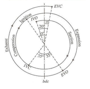
| Injection Timing | 120, 90, 60 DBTDC |
| Duration | 30, 40, 50 CA |
| Connecting rod length | 185.0mm |
| Maximum intake valve lift | 11.83mm |
| Exhaust valve opening | -236.0 BTDC |
| Exhaust valve closure | 14.0 ATDC |
| Intake valve opening | -21.0 BTDC |
| Intake valve closure | 231.0 ATDC |
| Engine speed | 1500, 2800 rpm |
| Swirl ratio (S/R) | 1.97, 3.73 |
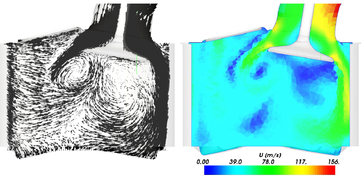
Flow field vectors and velocity magnitude at IVC or 600 CAD, plane cut through the middle of the intake valve and parallel to the symmetry plane. Reference of this image is: CFD modeling of a four stroke S.I. engine for motorcycle application by STEFAN GUNDMALM as Master of Science Thesis.
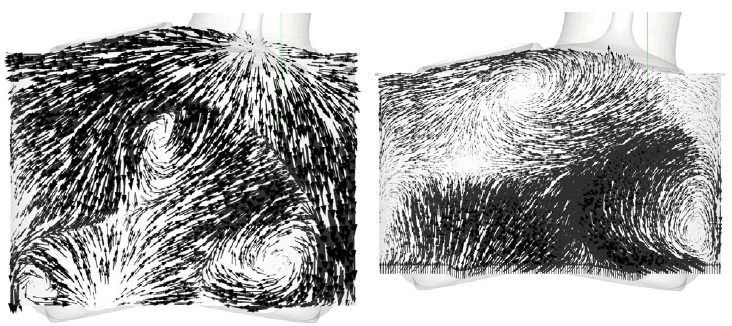
Flow field at BDC (540 CAD) and flow field at IVC (600 CAD), plane cut through the middle of the cylinder (the symmetry plane).
Data for Mercedes-AMG A45, Engine: M 133 DE 20 AL (reference - State of the art cooling system development for automotive applications, GT Conference 2017, Frankfurt)
- 4-cylinder engine, Displacement: 1991 cm3
- Output: 280 [kW] / 381 [hp]
- Max. Torque: 475 [N.m]
- Specific output: 140.6 [kW/liter]
- Heat input to cooling system ~ 200 [kW]
Wartsila-Sulzer RTA96-C turbocharged two-stroke diesel, built in Finland, used in container ships
- 14 cylinder version: weight 2300 tons (2,086,525 kg), length 89 feet (27 m), height 44 feet (13.4 m)
- Maximum power 108920 hp (81.25 MW) at 102 rpm, maximum torque 5,608,312 ft-lb (7605 kN-m) at 102 RPM
- Power/weight = 0.024 hp/lb (0.0709 kW/kg)
- One of the most efficient IC engines: 51%
| Honda GX35 engine |
| Bore x Stroke [mm] | 39 x 30 |
| IVO/IVC [BTDC/ATDC] | 25.41/66.21 |
| Displacement [cc] | 35.8 |
| Maximum valve lift [mm] | 2.82 |
| Intake air system | Naturally aspirated |
| Compression ratio | 8:1 |
| Intake valve lift [mm] | Angular interval [°] |
| 1.000 | 41.967 |
| 2.000 | 30.059 |
| 2.500 | 21.929 |
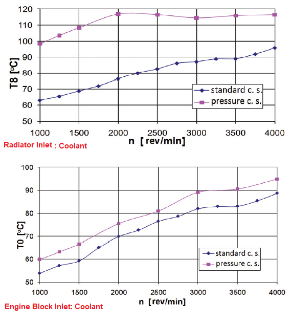
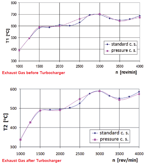
Reference: INFLUENCE OF SPEED AND LOAD ON THE ENGINE TEMPERATURE AT AN ELEVATED TEMPERATURE COOLING FLUID, Rafal Krakowski, Faculty of Marine Engineering, Morska Street 83, 81-225 Gdynia, Poland
Following data is for a four-cylinder engine with indirect fuel injection into the vortex chamber performed in the cylinder head.
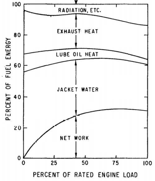
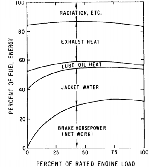
Heat balance for a 4-stroke gasoline (petrol or spark ignition engine): "Heat Balance of Modern Passenger Car SI Engines" by Gruden, Kuper and Porsche in
Heat and Mass Transfer in Gasoline and Diesel Engines, ed. by Spalding and Afgan.
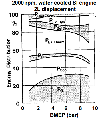
Power-flow diagram in internal combustion reciprocating engines:
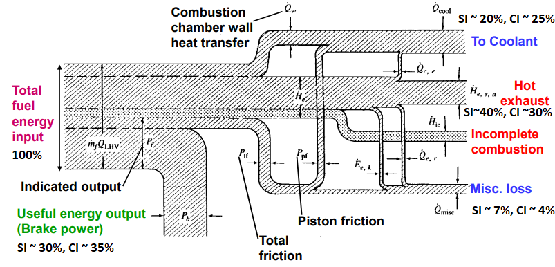
Order of Magnitude: SI engine peak heat flux ~ 1-3 MW/m2, Diesel (CI) engine peak heat flux ~ 10 MW/m2. For SI engine at part load, a reduction in heat losses by 10% results in an improvement in fuel consumption by 3% (based on the fact that 30% of the fuel energy is converted into useful power).
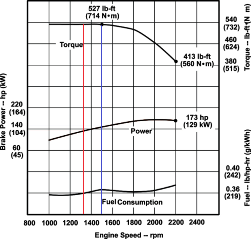
For a Diesel engine with following ratings:
- Rated power/Rated speed: 129 kW (173 hp) at 2200 [rpm]
- Peak torque: 714 N.m (527ft-lb) at 1500 [rpm]
- Power at peak torque: 112 kW at 1500 [rpm], 13% less than rated power. Depending upon the engine RPM, this drop in power at maximum torque conditions can be higher (up to 30%) as shown in following chart.
INTERNAL COMBUSTION PISTON ENGINES by Charles L. Segaser - ANUCES/TE 77-1, prepared by Oak Ridge National Laboratory: A generalized empirical equation to correlate part-load performance data of the engines is given by equation Y = A + BX + CX2 + DX3 where Y represents the value of a particular function, such as brake horsepower jacket water heat rejection corresponding to input values of the independent variable X which can be the % of rated load of the engine or other appropriate variable.
Generalized Equation Coefficients - Percent (Y) of Specific Fuel Consumption at Full-Load for Representative Large Gas, Dual-Fuel and Diesel Engines Vs Percent (X) of Rated Load (25 ≤ x ≤ 100)
| Engine | Coefficients |
| Type | A | B | C | D |
| 2-cycle gas | 506 | -10.9 | 0.098 | -2.96E-04 |
| Turbocharged 2-cycle gas | 558 | -15.1 | 0.168 | -6.30E-04 |
| Turbocharged 4-cycle gas | 219 | -3.74 | 0.041 | -1.54E-04 |
| Turbocharged 4-cycle gas-diesel | 176 | -2.51 | 0.028 | -1.09E-04 |
| Turbocharged 4-cycle diesel | 142 | -1.61 | 0.019 | -6.94E-05 |
Heat Balance - Turbocharged Low-Speed Compression Ignition Diesel Engine
Generalized Equation Coefficients - Distribution of Input Fuel Energy (Y, %) Vs % of Rated Load (X) for 4-Cycle Turbo-Supercharged Engines:
Coefficients for representative diesel engine heat balance curve:
| Engine | Coefficients |
| Parameters | A | B | C | D |
| Brake Thermal Efficiency | 0.00 | 1.449 | -1.869E-02 | 8.00E-05 |
| Jacket Water Heat | 43.0 | -0.886 | 1.114E-02 | -4.907E-05 |
| Lube Oil Heat | 12.0 | -0.194 | 1.143E-03 | 0.00 |
| Exhaust Heat | 39.0 | -0.159 | 1.714E-03 | -6.40E-06 |
Coefficients for representative gas and dual-fuel engines:
| Engine | Coefficients |
| Parameters | A | B | C | D |
| Brake Thermal Efficiency | 0.00 | 1.267 | -1.633E-02 | 6.867E-05 |
| Jacket Water Heat | 41.0 | 0.613 | 6.940E-02 | -2.662E-05 |
| Lube Oil Heat | 12.0 | 0.613 | 4.489E-03 | -2.026E-05 |
| Exhaust Heat | 32.0 | 0.232 | 3.438E-03 | -1.563E-05 |
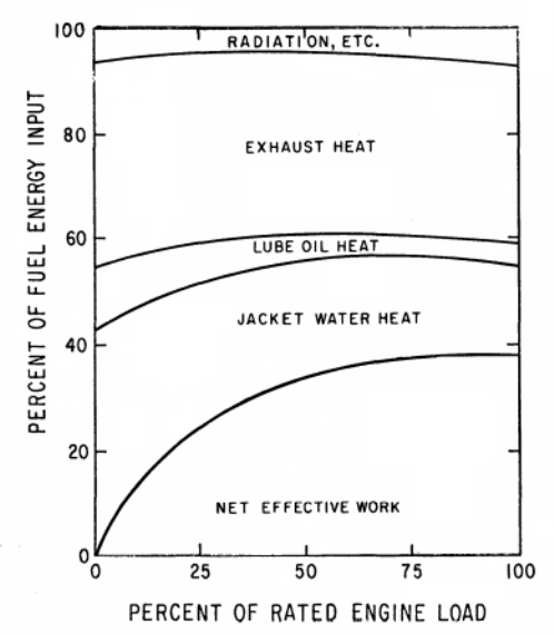
Heat Balance - Naturally Aspirated Spark Ignition Gas Engine with Hot Exhaust Manifold (no cooling of exhaust manifold)
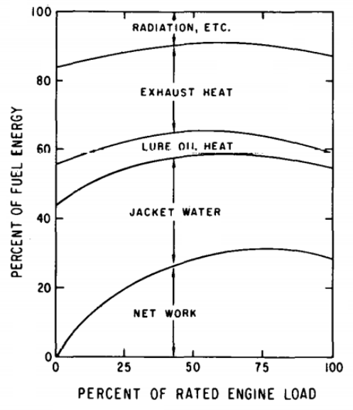
Heat Balance - Naturally Aspirated Spark Ignition Gas Engine with Water-Cooled Exhaust Manifold
Heat Balance - Turbocharged Spark Ignition Gas Engines: A certain amount of heat (approximately 3-16% of the heat input) will be radiated to the environment. The sum of all the losses plus heat rejections and heat converted to useful work must always add up to the total heat input at any engine load.
Thermal Efficiency of Typical Spark-Ignition Gas Engines
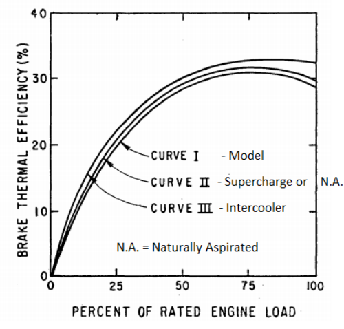
Generalized Equation Coefficients - Brake Thermal Efficiency of Spark-Ignited Gas Engines (Y) vs. a Percentage of Rated Load (X) where 0 ≤ X ≤ 100
| Engine | Coefficients |
| Parameters | A | B | C | D |
| Naturally aspirated with hot exhaust manifold | 0.00 | 1.0364 | -1.1052E-02 | 3.5880E-05 |
| Naturally aspirated with water-cooled exhaust manifold | 0.00 | 1.0976 | -1.2143E-02 | 4.1667E-05 |
| Superharged Intercooled | 0.00 | 1.2670 | -1.6334E-03 | 6.8866E-05 |
Jacket Water Heat Rejection - Typical Spark Ignition Gas Engine
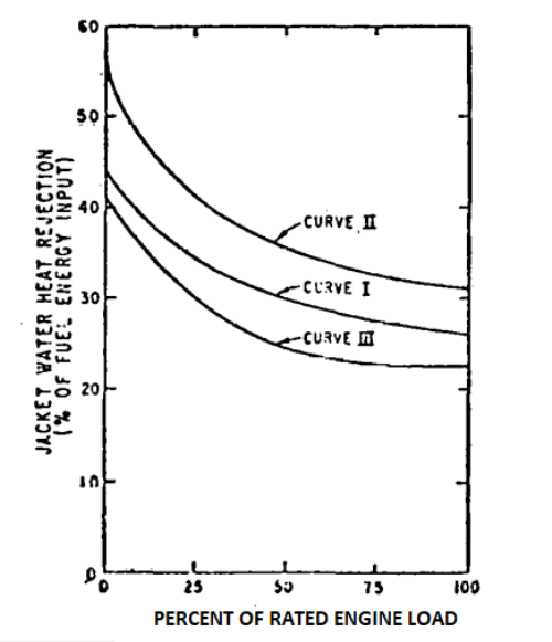
Generalized Equation Coefficients - Jacket Water Heat Rejection from Spark-Ignited Gas Engines (Y) vs. a Percentage of Rated Load (X) where 0 ≤ X ≤ 100
| Engine | Coefficients |
| Parameters | A | B | C | D |
| Naturally aspirated with hot exhaust manifold | 43.754 | -0.503 | 5.784E-03 | -2.546E-05 |
| Naturally aspirated with water-cooled exhaust manifold | 5.730 | -0.842 | 1.090E-02 | -4.977E-05 |
| Superharged Intercooled | 40.925 | -0.613 | 6.940E-02 | -2.662E-05 |
Exhaust Gas Heat Rejection- Typical Spark Ignition Gas.Engines: A considerable portion (~ 30%) of the toal heat input to gasoline engine is rejected to the exhaust, but only about 60~65 % of this heat can be recovered because it is necessary to maintain the exhaust gas at a temperature greater than 325 [°F] ± 25 [°F] or 163 ± 4 [°C] to prevent corrosion of the heat recovery equipment. The exhaust gas temperature of gas engines varies from approximately 800 ~ 1350 [°F] or 427 ~ 732 [°C] depending on the size of the engine, its efficiency and whether it is superharged and/or intercooled.
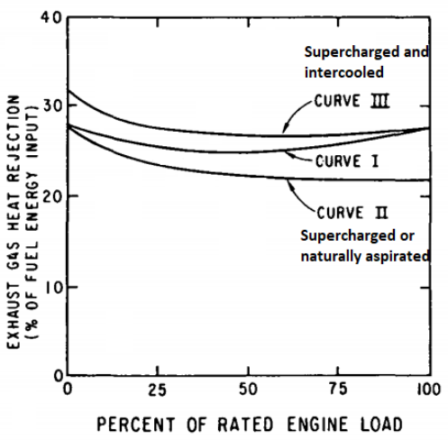
Generalized Equation Coefficients - Exhaust Gas Heat Rejection from Spark-Ignited Gas Engines (Y) vs. a Percentage of Rated Load (X) where 0 ≤ X ≤ 100
| Engine | Coefficients |
| Parameters | A | B | C | D |
| Naturally aspirated with hot exhaust manifold | 28.056 | -0.167 | 2.937E-03 | -1.273E-05 |
| Naturally aspirated with water-cooled exhaust manifold | 27.905 | -0.236 | 3.155E-03 | -1.389E-05 |
| Superharged Intercooled | 31.857 | -0.232 | 3.438E-03 | -1.563E-05 |
Generalized Equation Coefficients - Typical Diesel Engine Heat Balance (Y) vs. Percentage of Rated Load (X) where 0 ≤ X ≤ 100
| Engine | Coefficients |
| Parameters | A | B | C | D |
| Brake Thermal Efficiency | 0.00 | 1.449 | -1.869E-02 | 8.000E-05 |
| Jacket Water Heat | 43.0 | -0.886 | 1.114E-02 | -4.907E-05 |
| Lube Oil Heat | 12.0 | -0.194 | 1.143E-03 | 0.00 |
| Exhaust Heat | 39.0 | -0.159 | 1.714E-03 | -6.400E-06 |
| Radiation | 6.00 | -0.090 | 1.314E-03 | -2.667E-06 |
The exhaust gas heat rejection for the engine heat balance given in the table above was based on a flowrate of 12 [lb/Bhp-h] or 2.028 [g/kW/s] and an exhaust gas temperature of 855 [°F] or 547 [°C] at full load. For some highly turbocharged 4-stroke engines, the mass flow can be as high as 13 [lb/Bhp-h] or 2.196 [g/kW/s]. The temperature of the exhaust gas following the supercharger is variable, depending on the engine manufacturer but generally will be from about 650 ~ 855 [°F] or 343 ~ 547 [°C] at full load. At part load, the exhaust gas temperature decreases.
In Diesel engines, intake air not throttled, load controlled by the amount of fuel injected, A/F ratio: idle ~ 80, Full load ~ 19 (less than overall stoichiometric)
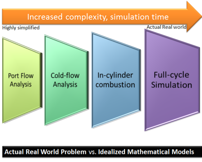
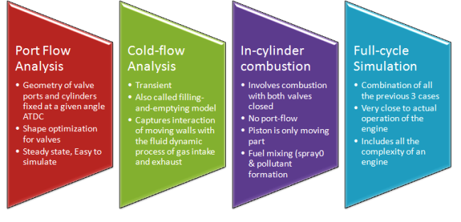
Simplifications and Stages of Numerical Methods
Engine Combustion
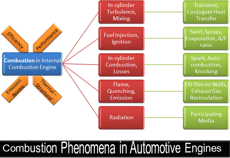
Combustion is a complex phenomena involving fluid flow, all three modes of heat transfer, structural severity, lubrication, emissions and very short duration phenomena. Typically, such simulations are performed in specialized programs such as KIVA. However, to gain deeper insight into the physics, CFD tools have now been widely and successfully exploited in a staged manner.
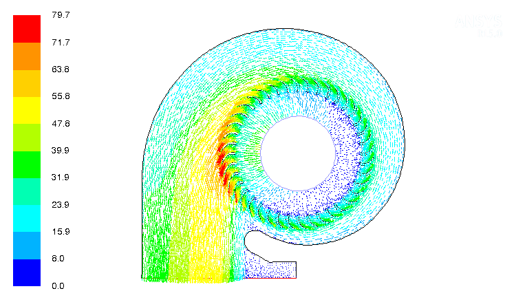
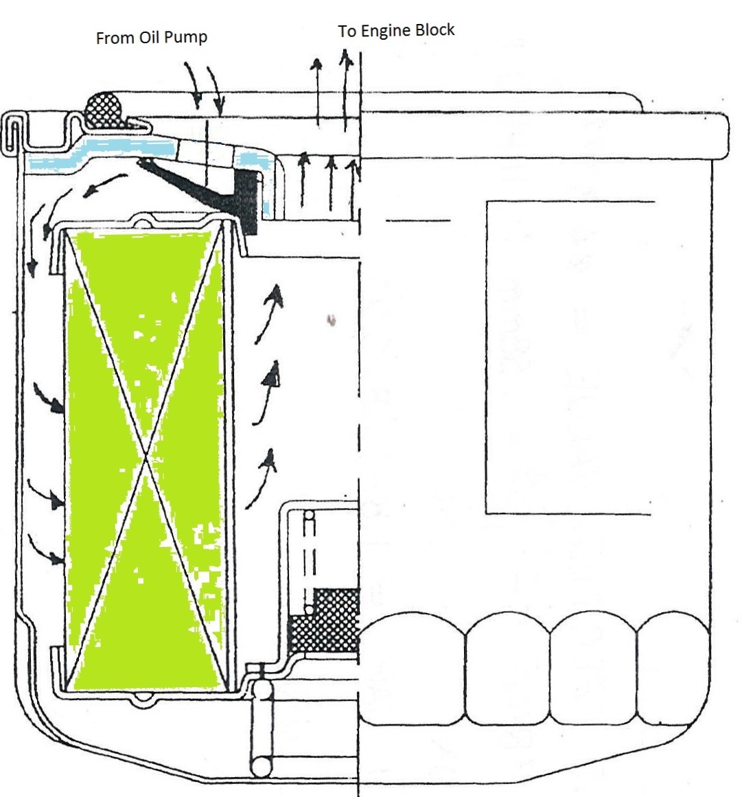
Oil Filter - Flow through Porous Domain
The performance of oil filter (pressure drop and flow uniformity across filter) can be optimized using numerical fluid dynamic calculations. The filter can be used as porous domain whose porosity can be varied as the particulate matters get trapped during actual use.
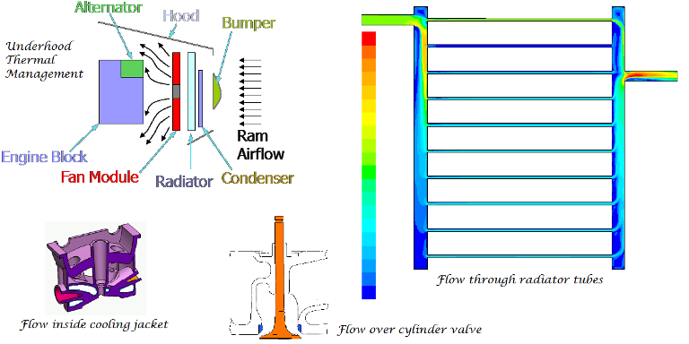
Component Level Appliations
There always exist a scope of improvement in the performance of individual components. The power of numerical simulations can be exploited without costly prototypes. For example, the location on inlet and outlets of a radiator is constrained by performance requirement as well as layout inside the engine compartments. The flow distribution inside the radiator tubes can be improved for different location of the inlet and outlet as well as shape and size of headers.
System Level Simulations: 1D
Applications of CFD at system level simulation are (a)complete cabin HVAC simulation and (b) engine cooling circuit simulation including water pump, cooling jacket in engine block and cylinder head, thermostat valve, radiator and associated plumbings. These simulations are complex in nature and the turn-around time is too high. At the early stage of design and development, a quick method is required where design iterations can be performed in a very short duration say < 1 day.
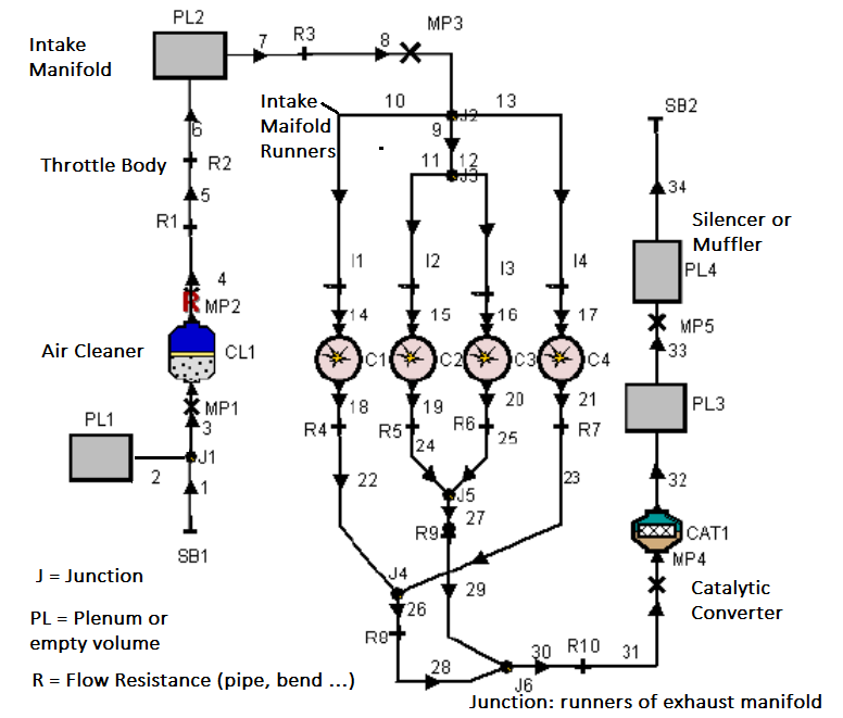
1D (1-Dimensional) simulation approach is intended to fill this gap - this method is also known as "lumped parameter approach" where a 3D geometry is represented as equivalent flow resistance and junctions. For example, GT-Power from Gamma Technologies , ALV-Boost from ALV or Ricardo Wave can be used to simulate complete air-flow path in internal combustion engines.
Similarly, applications like KULI ad FlowMaster can be used to make 1D calculation on the cooling systems such as HVAC. Following image describes the representation of a engine system that includes air intake from ambient till exit of combustion products into the atmosphere using program AVL-Boost.
Similarly, the 1D model for a single cylinder engine using GT-Power is described below.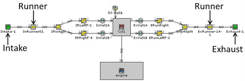
GT Suit provides option to create engine models with different level of complexity. For example, a very detailed simulation model known as full combustion model can be used to calculate characteristics of the working engine. This model is used to find or tune the engine to maximum performance (efficiency and/or power and/or torque) by varying different operational parameters of the engine. Howevver, this model is computationally intensive and may not be appropriate for all sorts of engine development works.
GT suite has a simpler model called the "mean value engine model" which is a simplified version of the full combustion model. As the combusion phenomena is approximated, the main difference between these two models is in the cylinder block object (e.g. 'EngCylCombSIWiebe' or 'EngCylCombDIWiebe). The mean value model uses the data obtained from the full combustion model without actually performing the actual combustion calculations. This is the best compromise between the accuracy and computational resources. Mean value model allows changing different parameters such as engine speed, fuel injection, air-fuel ratio, start of injection, variable geometry turbocharger (VGT) and exhaust gas recirculation (EGR) parameters.
The solution is NOT an iterative numerical process (as is the case in a most the numerical analysis such as 3D CFD simulations). The solution is based on the state of the system at time tn and is calculated for a new time tn+1. The new time tn+1 must close enough to time tn to ensure the solution is valid. This maximum time step is always calculated at each time step such that the Courant number is ≤ 0.8. Time step is calculated for each sub-volume (branch) and the smallest one is applied to entire system
GT-SUITE
This is collection of modules which comprises of six solvers (GT-Power, GT-Drive, GTVtrain, GT-Cool, GT-Fuel, and GT-Crank), a GUI GT-ISE, a post-processor GT-POST and other supporting tools. The graphical user interface (GUI) to build models as well as the means to run all GT-SUITE applications is GT-ISE. The thermodynamic modeling program for engines, GT-Power is available as a standalone tool or coupled with GT-Drive, GT-Fuel and GT-Cool as the GT-SUITE / flow product.
This program is based on library of lumped objects classified into 4 types.
- Component objects: these objects refer to individual parts which are simple flow resistances such as pipes, bends, valve, inlets, exits...
When modeling the comopnents, close attention to any point of area change is required. These geometrical features are large source of pressure drop in typical manifolds, pressure waves are reflected off these area changes due to the change in velocity. The reflection of waves is important to manifold wave dynamics, both for performance (breathing) and acoustic
results.
- Reference objects: This category of objects are not related to physical layout but the operational data and material properties such as Air-Fuel ratio, reference temperature and pressure, looup tables,fan map, liquid properties and other boundary conditions. These objects cannot be placed on the 1D map but are directly linked to component and compound object types.
E.g. Fuel Injection - InjProfileConn for profile injection which is used in direct injection and required inputs such as fuel mass per stroke, vaporized fuel fraction, injection rate vs. crank angle, nozzle discharge coefficient
(between 0.65 and 0.75). Additionally, smoke-limits may be imposed. InjAF-SeqConn - sequential fuel injection used in sequential port injection requires injector delivery rate (Air Fuel Ratio, Start of Injection, Vaporized fuel fraction). This object is ideal for developing fuel maps and vaporization effects on volumetric efficiency can be modeled more accurately.
- Compound objects: these are sub-assemblies of the system such as the engine itself.
- Connection object: To connect different parts of the model together links should be created. Two parts are usually connected by a link and a connector part that is inherited from a connection object. A connection object must correspond to the way two parts are connected to each other. Every object has a number of ports that can be used for the connection. The description for the ports can be found by double-clicking the arrow linking objects.
Component objects
- Pipe: This object of standard library represent straight pipe of uniform or varying (tapered) cross-section. Roughness can be accounted for calculating friction factor.
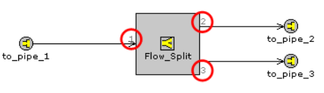
- FsplitTRight: It refers to Flow-Split at Tee-Junction when flow goes into only one side branch (Right-branch here).
- FsplitSphere: Flow split spherical junction.
- FsplitGeneral (say Wye- and X-junctions): Flow-split of generic type where users can specify angle of merging and diverging streams.
- PipeRoundBend: Uniform bend such as elbow bend, S-bend
- ValveCamPR: This object is similar to ValveCamConn' except that forward discharge coefficient (flow at inlet ports) and reverse discharge coefficient (flow at exhaust port), swirl (helical flow inside the cylinder), and tumble can be defined as functions of both stroke/bore ratio and compression pressure ratio. Also, there is an option to make these coefficients functions of L/D and piston-position.
- ValveCamConn: connection to valve and camshaft which drives the valves, the valve-lift vs. Cam angle is specified and corresponding flow characteristics (discharge coefficients) need to be defined.
- Exval: Exhaust valve
- EngCylinder: Engine cylinder usually represented by bore and stroke length and refer to several reference objects for modeling information on combustion and heat transfer.
- EnegineCrankTrain:
- EndEnvironment: Ambient condition into which the combustion products finally gets discharged after passing through silencer.
- Air Boxes: These are thos parts of the engine with cross-section area significantly larger than the entering and exiting pipes and can be made irregular in shape due to space constraints. The components such as Helmholtz resonator and plenum of intake manifold are air boxes. Such air volumes and air cleaner assembly have significant effect on intake system pressure drop and acoustic behavior, and is therefore an important part of the engine model.
Reference objects
This group of objects contain different types of data that are used in the simulation models for example lookup tables, boundary conditions, functions, liquid properties ...
- FPropMixtureComb - Air:
- FStateInit - Init:
- HeatCComp - ExhManifold:
- RLTDependence - FARatio:
- FPropLiqInComp - Indolenecombust:
- XYTable (FARvsRPM, THB50vsRPM, BDURvsRPM):
- XYZTable - INTPr:
- FPropGas - Indolene-vap:
- Many attributes and options in GT-ISE can be parameterized by adding a variable name in square brackets to the entry field instead of typing in value in numerics. All these parameters for the active model are defined at the case setup available from menu or can be accessed by pressing F4.
Compound objects
- Engine: the engine assembly which includes combustion chamber
- CrankTrain: It represents connection rod, crankshaft, bearing journals, connecting rod pin, piston, piston rings.
Connection objects
In a GT-Power model, black lines represent actual physical connections like a pipe bends and a pump connected to each other with the coolant flow going from the first component to the second one or the heat being transferred from one side of the heat exchanger to another. On the other hand, blue lines represent signal and sensor connections, they allow to extract different types of data from the model like temperature, mass flow or volumetric flow.
- Orifice Conn - bellmouth: inlet to pipes
- InjAF-Ratio Conn: Air-fuel ratio for injectors used typically to model a carburetor or fuel control valve on SI engines. It injects fuel at a constant fuel-to-air ratio.
- InjAFSeqConn: This injector connection is used to model sequential fuel injection in SI gasoline engines. This injector would be used when one knows the injector delivery rate and the desired fuel ratio. An important output of this injector is the calculated pulse width.
- ThrottleConn - throttle: connection objects for throttle body, required to specify throttle opening.
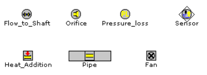
- Orifice, Pressure_Loss, Sensor
- Flow_to_Shaft: Output to shaft connected to the engine.
- Valve*Conn (ValveCamConn, ValveCamPRConn, ValveCamDesignConn, ValveCamDynConn, ValveCamUserConn and ValveSolenoidConn): This type of connection object is used to connect cylinders to intake and exhaust ports.
Note:
Like any other numerical methods, simulation model needs to be validated against experimental data. In 1D calculations also, there are many uncertainties about the pressure losses, temperature of walls, hot air recirculation, RAM effect of moving object, mixing losses at junction ... on the air side of the system. Thus, every such model requires initial tuning.
The value for the heat input rate from the engine block can be directly extracted from the engine cylinder mean value object (EngCylMeanV). The output variable is called "Heat Transfer Rate". The value is in [W] which needs to be multiplied by 1000 to obtain data in [kW] needed as an input to the EngineBlock object of the cooling system model.
To calculate the heat load for oil cooler, there is no direct approach and method of energy balance needs to be used. The heat load on oil cooler is mostly the heat generated by friction in piston rings and liner. Thus, in order to calculate the heat load on oil cooler, the friction torque should be calculated. For this purpose a MathEquation object can be used. "Inst. Indicated Torque" and "Inst. (Indicated-Friction) Torque" can be extracted from the "Crankshaft object" of the mean value model which can then be used to calculate friction torque [N-m] = "Inst. Indicated Torque" - "Inst. (Indicated-Friction) Torque". Since power = torque × angular speed (ω), friction power = friction torque × angular speed = heat load on oil cooler.
The fan performance in GT-Suite is dependent on the fan speed, even for the free-wheeling or wind-milling conditions when ram air drives the fan and not the motor. The fan speed always be directly defined by the user and there is no mechanism to calculate fan speed automatically. Defining fan speed as zero makes this component work as a blockage not allowing any air to flow through. Hence, to model fan-off conditions it is recommended to set the fan speed to some guess value that will correspond to the speed of fan under wind-milling condition.
References: Cooling performance simulations in GT-Suite: Master’s Thesis by ALEXEY VDOVIN, Department of Applied Mechanics, Division of Vehicle Engineering and Autonomous Systems, Chalmers University of Technology, 2010
Fundamentals: Working Principle and Design Ratios
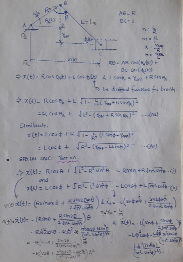
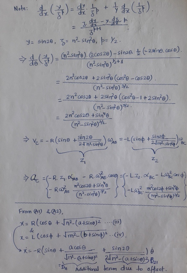
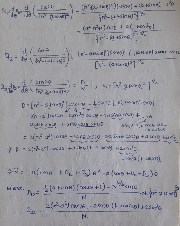
The conversion of rotating motion to translating motion using a slider-crank mechanism is explained in the following figure. The locus of some of the points which is translating as well as rotating is also shown.
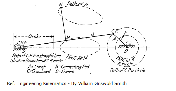
- Length of the stroke = diameter of the crank pin = DCP. Piston travel per revolution = 2 * DCP. Distance traveled by crank pin per revolution = π * DCP. Hence, the ratio of average piston velocity to that of crankshaft pin = 2 * DCP / π * DCP = 2/π.
Slider Crank Mechanism Animation
The Octave script used to create this animation is as follows:
clc; clear;
% Define constants - use consistent units: mm, rad, s
  N =   5;               % [rpm] - crankshaft rotation speed
  R     =   0.075;           % [m] - Crank Radius
  L     =   0.200;           % [m] - connecting rod length
  w     =  2*pi*N/60;        % [rad/s] - angular speed
  tau   =  2*pi/w;           % Time for one complete rotation of crankshaft
  dq    =  pi/30;
  Lp    =  0.010;            % Piston Length
  Db    =  0.020;            % Bore diameter = piston diameter
%------------------------------------------------------------------------------
% Define parameters, calculate functions and plot
%
  x(1)  = 0.0;
  y(1)  = 0.0;

  xMax  = L + 2*R + Lp; xMin = -2*R;  yMin = -2*R; yMax  = 2*R;
  figure;     axis([xMin xMax yMin yMax]);     hold on;     daspect([1 1 1]);
  plot(x(1), y(1), 'o');
  for q =  [0: dq : 2*pi]
    x(2)  = R * cos(q);
    y(2)  = R * sin(q);
  % Location of piston centre with crank angle q.
    x(3)  = R * cos(q) + sqrt(L^2 - R^2 * sin(q) * sin(q));
y(3)  = 0;
x(4)  = x(3) - Lp/2.0; y(4) = 0.0;
x(5)  = x(4);          y(5) = -Db/2.0;
x(6)  = x(3) + Lp;     y(6) = y(5);
x(7)  = x(6);          y(7) = y(6) + Db;
x(8)  = x(4);          y(8) = y(7);
x(9)  = x(4);          y(9) = 0;
  %
  % Time derivative of x - excluding q_dot term
    n     = L/R;
    xp    = -R * sin(q) - R * sin(2 * q) / sqrt(n^2 - sin(q) * sin(q) );
  %
  % Piston velocity
    V     =  xp * w;

    plot(x(2), y(2), 'o'); plot(x(3), y(3), 'o');
    plot(x, y, "linestyle", "-", "linewidth", 2, "color", 'k');
    xlabel('x'); ylabel('y');
    %grid on;  % should be placed only after the plot command
    xtick = get (gca, "xtick");
    xticklabel = strsplit (sprintf ("%.2f\n", xtick), "\n", true);
    set (gca, "xticklabel", xticklabel)

    ytick = get (gca, "ytick");
    yticklabel = strsplit (sprintf ("%.2f\n", ytick), "\n", true);
    set (gca, "yticklabel", yticklabel);
    pause (0.0001); cla;  plot(x(1), y(1), 'o');
    axis([xMin xMax yMin yMax]); daspect([1 1 1]);
  end
  plot(x, y, "linestyle", "-", "linewidth", 2, "color", 'k');
  plot(x(2), y(2), 'o'); plot(x(3), y(3), 'o');
Combustion
Combustion is on the most complex thermo-chemical phenomena known to us. This is much more than fluid mechanics and heat transfer and hence a typical method of CFD simulations does not fulfill the requirements. The complexity of combustion is described by following slides.
Types of Combustion
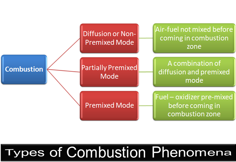
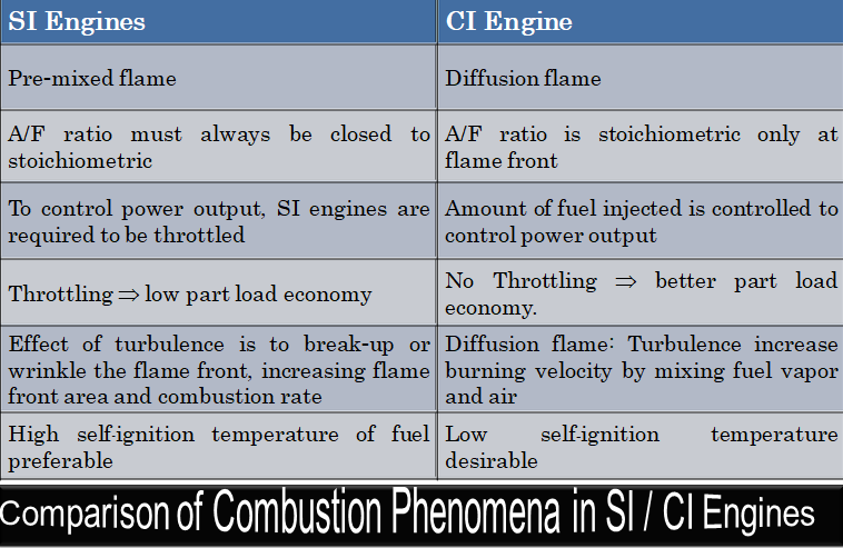
Non-Premixed Combustion

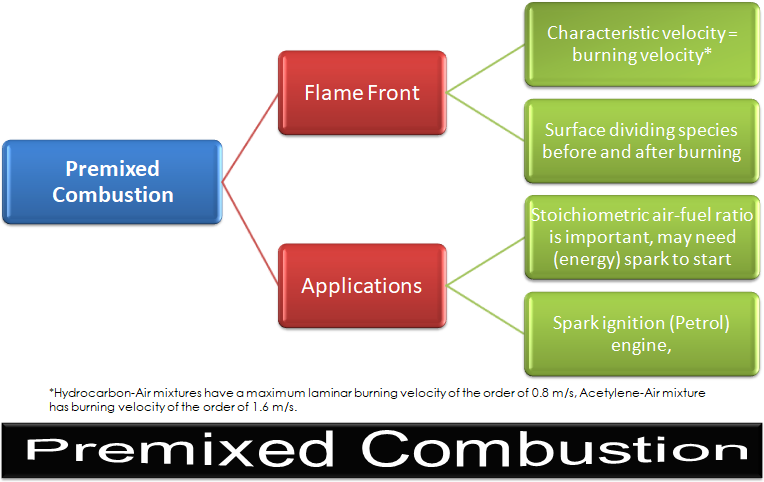
Premixed Combustion
Combustion modeling of diesel fuel requiresespecially and complex modeling such as sub-models for turbulence, spray injection, fuel atomization / breakup, coalescence, vaporization, ignition, premixed combustion, diffusion combustion, radiative + convective heat transfer and emissions (soot and NOx). All of these sub-models must work together in turbulent flow fields. CFD modeling requires fine spatial resolution for processes like local auto-ignition and rolling up of flame surfaces.
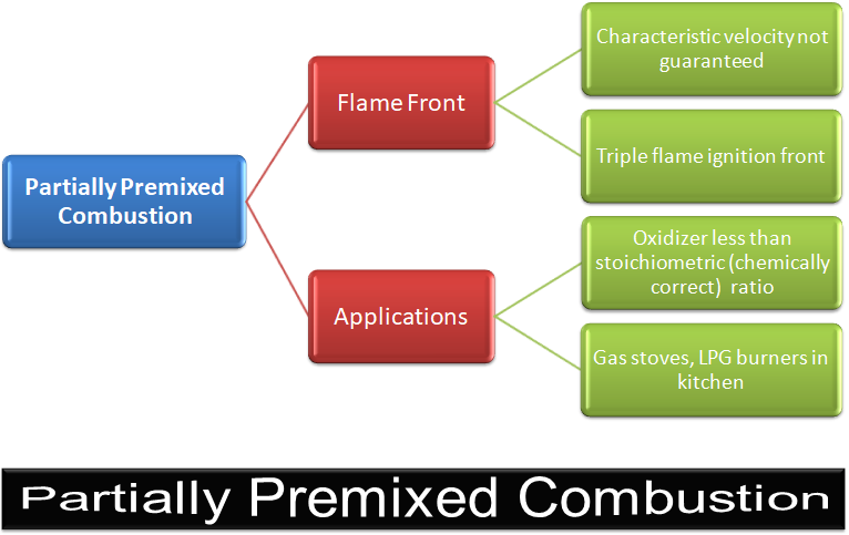
Partially Premixed Combustion
Combustion Phenomena in Engines
Combustion: CI vs. SI Engines
Application of CFD in Gearbox Applications
CFD can be used to check lubrication of gears, rise in temperature due to viscous heating of oil, splashing of oil from rotating teeth and churning losses. The multi-phase flow simulation using dynamic and deforming meshes is required to capture the phenomena of oil squeezing between gear teeth and spillage as gear teeth emerges from oil bath. A useful video on this topic is "youtube.com/watch?v=NCrtWr74f4c". A screenshot from the video is shown below: 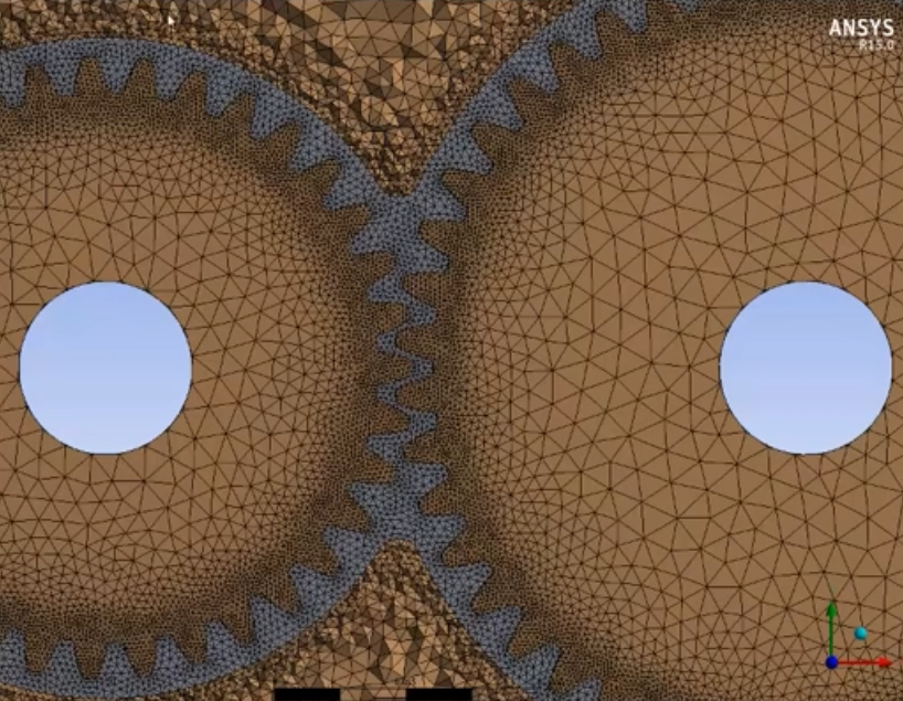
Power losses in gearboxes are of tow types: (1)Load dependent: those caused by the loads being applied: friction in gear engagement and friction in bearing parts (2)Load independent which are not dependent of loads applied: such as shaft seal and churning losses.
The churning losses arise due to gears temporarily moving into the oil and it primarily is function of depth of oil immersed. The churning loss can be as high as same order of magnitude as gear friction losses whereas seal power loss is an order of magnitude lower than the gear friction losses.
Excerpts from papers available on internet
Defrost and Defogging / Demisting: 'Frost' means formation of a layer of ice in cold condition right across the outside face of the wind screen. 'Mist' means a film of condensate on the inside face of the glazed surfaces. Condensation is formed as small water droplets and can be seen as fog. A system responsible for removal of frost is called as defrosts system and system responsible for removal of mist is called as demist system.
Modern LED headlamp in comparison with previously used halogen lamps generate or radiate lesser fraction of input power as heat. While halogen lamps would heat the front glass of the headlamp by infrared radiation, the waste heat created in LEDs is mainly conducted away into heat sinks which are placed in the back of the lamp or even outside. This makes the front glass of the new lamps more prone to fogging.
Water film (fog) that forms on the windshield during winter times and reduces adriver’s visibility, originates from condensing water vapor on the inside surface of the windshield due to low outside temperatures. Primary source of this vapor is the passenger’s breath which condenses on the windshield. The passenger cabin of an automobile contains air with a relevant content of water vapors, originating from various sources (breath of passenger(s), outside humidity, wet hair, wet clothing, wet mat). These vapors condense on the inside surfaces of the cabin, especially on the windows (windshield, side windows, rear windows), due to lower temperatures of the outside air and radiation heat transfer effects.
The paper "CFD Simulation of Defogging Effectivity in Automotive Headlamp" by Michal Guzej and Martin Zachar from Brno University of Technology, Faculty of Mechanical Engineering, Czech Republic provides good insight into the fogging mechanism and thermal simulation approach for defogging. Other papers describing the condensation and defogging methods are: "Condensation Zone Estimation and Determination and Comparison of Condensation by Numerical Analysis in Vehicle Lighting System" by Kemal Furkan Sökmen et al, "CFD Modelling of Headlamp Condensation" - Master’s Thesis in Automotive Engineering by JOHAN BRUNBERG at CHALMERS UNIVERSITY OF TECHNOLOGY.
The condensations phenomena inside an automotive headlamp can simply be explained by the inner surface of the transparent lens having a temperature equal to or above the current dew point of the air adjacent to the lens. This usually occurs locally around the lower edge of the lens and slowly grows upwards depending on how severe the circumstances are. Most analysis on the subject simplifies the condensation on the inside of the lens as film condensation and so will also be the case in this thesis work. It is also considered conservative to assume film condensation.
For condensation to be able to occur, the moist air has to come into contact with a cold surface. The coldest surface in the headlamp is usually some areas on the outer lens which offers poor insulation against the environment, heat is also more easily dissipated through the transparent material. The lens therefore gets cooled quickly and provides the heat transport necessary to cool the lens and adjacent air below the dew temperature. Energy is also being released from the water vapour when it cools to liquid and that energy is quickly transported away through the lens. Some areas of the lens are however warmed by radiation from the lamp and by the flow of air that has been warmed by the lamp. The temperature variations on the lens result in a certain pattern where condensation is more likely to form.
The condensation can be solved either by using the Eulerian wall film (EWF) approach or Volume-of-Fluid (VOF) approach. EWF predicts the creation and flow of thin films of liquids on a surface. This approach assumes that the film thickness is much smaller than the radius of curvature of the surface. EWF allows only one condensable component, which can be water in automotive headlamp fogging. For computing simulations with thin liquid layers, the volume of fluid method (VOF) can be used, but this approach has a high computational power demand.
- Definition-1: The fog layer smaller than 5 micrometer [0.005 mm] is considered as transparent.
- Definition-2: The minimum dew thickness still considered as fogged was 0.1 [nm], which is the minimal visible light scattering thickness - [Curcio, J.A.: Adsorption and Condensation of Water on Mirror and Lens Surfaces; U.S. Naval Research Lab.: Washington, DC, USA, 1976] cited in "CFD Simulation of Defogging Effectivity in Automotive Headlamp" by Michal Guzej and Martin Zachar.
- The fog layer thicker than 200 micrometer [0.2 mm] might result in drips and run offs. To study fog layers of that thickness, two-phase flow analysis is required.
- 10 layers of prisms needs to be created in boundary region with first layer initial height of 100 micrometers [0.1 mm] - the one next to the window shells, the height of these prisms has to be exponentially increased based on a growth rate of 1.1. Thus, tenth prism layer height which will attach to the tetras will be 0.1 * 1.19 = 0.2358 mm.
- Fogging / Misting: During the simulation, the solver tracks the water vapour content throughout the computational domain. The following assumptions are applicable to this approach regarding the water condensation on the walls:
- Water film is a continuous film of condensed water on a wall, contained in the first cell next to the glass
- Surface tension, gravity effects are neglected on the water film
- Water film is not flowing or moving at any time
- Evaporation/condensation will happen at specified walls only
- Water vapour is at saturation conditions at the interface between the fog layer and moist air
- Condensation mass transfer rates are determined only by the gradient of water vapour mass fraction in the cells containing the condensation film
- The condensation film is stationary
- The inlet relative humidity is constant in time
- Gravity and surface tension effects of the condensation film is neglected
- The diffusion coefficient of water vapour in moist air is known as a function of local pressure and temperature, Mollier chart or the Bahrenburg approach
- Inlet and outlet mass flow rates of water vapour is much higher than the mass transfer through condensation
- For the film temperatures of above 0°C, water will appear on the glass surface. While film temperatures below 0.1 [°C] may cause ice formation and for the film temperatures in the range of −0.1 to 0 [°C], it is assumed that either freezing or thawing occurs and thermophysical properties at this temperature range is achieved by interpolation between values of ice and water.
- The solver delivers temperature, pressure and humidity for the cells next to the walls. The solver defogging calculation determines the mass transfer process and direction based on the following criteria:
- Evaporation when TCELL > TSAT, deficit in specific humidity as compared to dew point.
- Condensation when TCELL < TSAT, excess in specific humidity as compared to dew point.
- Equilibrium (no mass transfer) when TCELL > TSAT and excess in specific humidity or TCELL < TSAT and deficit in specific humidity.
- Defogging module determines the mass transfer rate by a diffusion law for specific humidity.
- Defogging module updates water film thickness based on the new mass transfer rate determined above.
- Defogging module applies appropriate source/sink to the water vapour species in the cells next to glass.
- Defogging module computes latent heat of vaporization/condensation and updating thermal boundary conditions to the solid/fluid sides of the glass.
Defrosting / Deicing
The defrosting model assumes that the melted ice run-off the system and does not re-coagulate into ice. Defrosting analysis is a two step process: steady state analysis to establish initial flow field and then transient temperature field using convection and conduction through glass. Enthalpy-porosity based solidification-melting model is used to model the melting of ice. The ice layer is modeled as an ice-water mixture with both solidus and liquidus temperature specified. The standard CFD procedure for such a problem is to first obtain a steady state constant temperature solution, then freeze the flow field and solve for only energy in unsteady state. Thickness of first boundary layer = 0.001 [mm]. Frost thickness needs to be set at t = 0, typical value is 0.5 [mm].
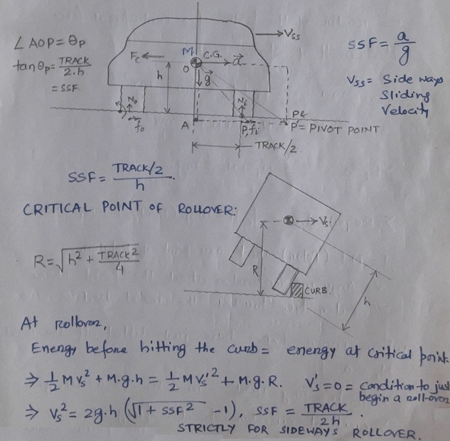
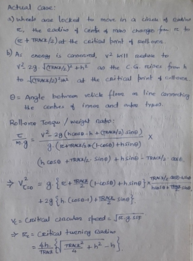
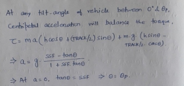
Car Roll-over Calculation
Skidding and sliding on an inclined plane: 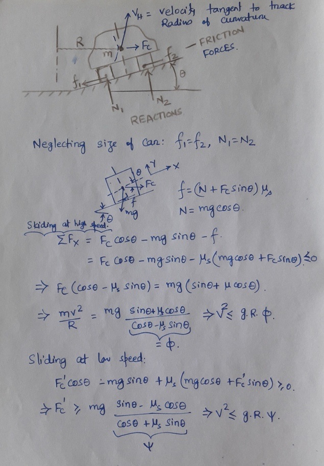
Static Stability Factor: SSF is defined as ratio of the "half of track width" and "height of the vehicle C.G.". There track width is transverse distance between centre of the tires. In other words, SSF is a lateral acceleration in multiples of 'g' at which roll-over may occur whn the vehicle is represented by a rigid body without suspension movement or tire deflections.
Roll-over on a circular path
Assumptions:
- Two inner tires towards the centre of the circular track are treated as one and ditto the other tires.
- Tires are not slipping, centripetal acceleration is constant.
- fi and Ni: friction and reaction forces on inner tires
- fo and No: friction and reaction forces on outer tires
- r = radius of the track, fc = centrifugal force, μs = coefficient of static friction
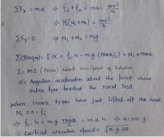
Note: centrifugal force is experience only by the car and not observed from outside of that frame of reference. In car was to disengage from the road, it would not be thrown towards outside of the track as the direction of centrifugal force will imply. Rather it would travel in a straight line along a direction tangent to the arc of the turn - in the direction of the mass inertia of the car at the points the car disengage / skid from the road.