- CFD, Fluid Flow, FEA, Heat/Mass Transfer: Feedbacks/Queries -
CFD Simulations in OpenFOAM
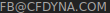
Open-source CFD toolbox
OpenFOAM is now a mature open-source CFD program with reliability matching that of commercial products. This page describes summary of utilities and dictionaries used in OpenFOAM meshing and visualization such as (blockMesh, snappyHexMesh, ParaView) and OpenFOAM CFD codes and pre-processors such as (simpleFoam, pimpleFoam, engineFoam...).
OpenFOAM CFD: A Beginner's Diary
Disclaimer:
This content is not approved or endorsed by OpenCFD Limited, the producer of the OpenFOAM CFD software and owner of the OpenFOAM and OpenCFD trademarks.Table of Contents: OpenFOAM workflow || Step-by-step Guide for OpenFOAM simulations |\/| mapFieldDict |/\| Post-processing Utilities and functionObjects || Data Interpolation |=| Porous Domains |=| Contact Resistance (*) Example blockMeshDict |:| Parametric blockMeshDict |+| Boundary conditions: Parabolic Velocity (*) Field Functions /-\ Boundary conditions: Fan {*} Wildcard characters
At the outset, start with few excerpts from User Guide: "OpenFOAM is first and foremost a C++ library, used primarily to create executables, known as applications. The applications fall into two categories: solvers, that are each designed to solve a specific problem in continuum mechanics; and utilities, that are designed to perform tasks that involve data manipulation. One of the strengths of OpenFOAM is that new solvers and utilities can be created by its users with some pre-requisite knowledge of the underlying method, physics and programming techniques involved. OpenFOAM is supplied with pre- and post-processing environments. The interface to the pre- and post-processing are themselves OpenFOAM utilities, thereby ensuring consistent data handling across all environments." Wikki Ltd is provider and major contributor to foam-extend, the community version of the OpenFOAM software. As per "Aerodynamic Shape Optimization of a Pipe Using the Adjoint Method" - IMECE2012-89396: OpenFOAM is a non-staggered Finite Volume Method code written in C++ using object oriented approach.
How many of these names have you heard of? Click the names to know more about them!

This open-source CFD code is released under GPL (GNU Public License), the product is free (free as in Toll-Free numbers, free-will, free-fall and free-wheel mechanism), powerful but comes with its own 'inconvenience'. Though the authors and programmers try their best to document everything, it still requires additional things to be learnt other than CFD itself, such as:
- complier and build-platform (such as "Windows XP Professional, Service Pack 2, 64-bit") used to prepare the binaries
- 'make' utility to compile the source codes, associated intermediate program like Qt, Cygwin
- Windows versions of required program such as "Visual Studio 2008 x86 9.0.30729.1 SP"
- Jargons like Kubuntu (Ubuntu + KDE) are by no mean kind to those either not familiar with Linux or not up-to-date with this OS!
- Yet, one can do with it whatever (s)he likes, including unlimited commercial use, serial or parallel computing.
- Installation: Linux - Ubuntu
- OpenFOAM for Windows by CFDSupport
- BlueCFD OpenFOAM version for Windows
- GeekoCFD: based on 64-bit Linux Platform openSUSE
- swak4Foam (Swiss Army Knife For Foam)
- The packages have been designed to allow simultaneous installation of different OpenFOAM versions without file or package-name collisions.
- openfoam.org and openfoam.com have different naming conventions for release versions. OpenFOAM from openfoam.org is installed in /opt/openfoam11 folder and applications from openfoam.com gets installed in /usr/lib/openfoam/openfoam2412 folder.
- Add following 4 lines in $HOME/.bashrc file where . at the start of lines can be replace by 'source'. The first two lines set the environment variables when a new terminal is opened and the last two lines create shortcuts to invoke desired version of OpenFOAM.
- . /opt/openfoam11/etc/bashrc
- . /usr/lib/openfoam/openfoam2412/etc/bashrc
- alias of24='source /usr/lib/openfoam/openfoam2412/etc/bashrc'
- alias of11='source /opt/openfoam11/etc/bashrc'
A set of tutorials explained in a step-by-step manner can be found in this pdf file.
Few troubleshooting and best practices can be found out at:- Few excellent videos on YouTube, by Jozsef Nagy, are: youtube.com/watch?v=Ds0eK1wXMks for blockMeshDict and youtube.com/watch?v=8J59CpaYnVc for OpenFOAM results in ParaView. Many thanks Jozsef!
- OpenFOAM uses its own makefile 'wmake' which is based on standard 'make' utility. However, the common 'makefile' command 'make' will not work with compilation of OpenFOAM codes.
- If you know what to look for, it is a great tool. If you don't, you might get lost in the hugeness of the OpenFOAM! The trick is to go through as many tutorials as possible and as many repeats you can make. You will find it worth doing.
OpenFOAM workflow
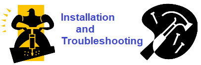
The simulation activities using OpenFOAM is a mix of commercial and open-source tools. Especially, the pre-processing such as creation of water-tight geometry and surface mesh (STL format) is easier outside open-source environment. The workflow without interaction with other program such as data exchange for structural simulations is described below.
The workflows that require interaction with other program such as data exchange for structural simulations shall require data interpolation and conversion as per the format required by them. For example, data export to ABAQUS or ANSYS format may require conversion of OpenFOAM data directly to the format recognized by these program or use of an intermediate format (such as FLUENT or I-DEAS) which ABAQUS or ANSYS can read.
Few key attributes
- OpenFOAM stands for: Open Field Operations And Manipulation. The word 'Open' can be thought to represent "Open Source CFD". FOAM is second part of the acronym which describes the numerical method to solve fluid dynamics problems.
- It is primarily, similar to CFX, a 3D-solver, hence all 2D meshes need to be extruded in third dimension. 2D problems are solved using special patches "empty". Excerpts from user guide: "OpenFOAM always operates in a 3-dimensional Cartesian coordinate system and all geometries are generated in 3 dimensions. OpenFOAM solves the case in 3 dimensions by default but can be instructed to solve in 2 dimensions by specifying a special empty boundary condition on boundaries normal to the (3rd) dimension for which no solution is required."
- It is a collection of Utilities, Solvers and Libraries based on programming language C++
- Utilities are specific functions needed to be performed in any CFD simulations such as "Mesh Generation and Checking", "Mesh Conversion", Post-processing...
- It is primarily a command line based solver, with less emphasis on GUI. It uses ParaView or paraFoam as post-processor.
- Paraview is a general-purpose post-processing tool to process many variety of formats.
- ParaFoam was a customized-version of Paraview to post-process results produced by OpenFOAM in its native format (i.e. without any interim conversion of data)
- Units of variables in OpenFOAM are specified as row vector of size 1x7 comprising of indexes [a b c d e f g] designated as [Massa Lengthb Timec Temperatured Quantitye Currentf Luminous Intensityg] which in SI unit is [kga mb sc Kd kilo-molee Af Cdg]. For example, the unit of dynamic viscosity, kg/m-s or Pa.s can be specified as [1 -1 -1 0 0 0 0].
- The solvers are named based on certain features and can easily be decoded and remembered after working through once or twice: For example, icoFoam is InCOmpressible Foam (icoFoam), simpleFoam is Semi-Implicit Method for Pressure-Linked Equations Foam...
- "SnappyHexMesh" or sHM in OpenFOAM is similar to "Cartesian Meshing" in ICEM CFD, "Trim Mesh" in STAR CCM+ and "Cut-cell method" in some other pre-processors. It generates a hexahedral mesh with hanging nodes.
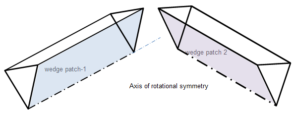
- Simulation of axi-symmetric flow problems, patch name 'wedge' is used. The wedge (also called prism mesh in other programs) is created by collapsing a pair of nodes - to convert a cuboid into a wedge - as described in the user manual shipped with OpenFOAM. Note that blockMesh will not work if wedge angle is > 15°.
- Files have free form, no need to indicate continuation across lines, no constraints on start column and end column
- // is used to put comment in OpenFOAM dictionary files, inline with C++ programming syntax. Comment encompassing multiple lines need to be enclosed between /* and */ delimiters.
- The OpenFOAM solver supports polyhedral meshes. It is believed that OpenFOAM had it first than any other program!
- The word patch in OpenFOAM refers to any 'boundary'
- Pre-processor Harpoon can directly export data in the native format of OpenFOAM (no data conversion required).
![]()
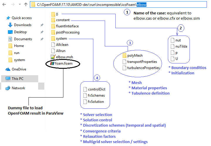
- Get version of OpenFOAM: utility 'foamVersion' shall print 'OpenFOAM-11' and echo $WM_PROJECT_VERSION shall print just '11'. blockMesh -help shall print "Using: OpenFOAM-11 (see https://openfoam.org)" at the end of output. echo $WM_PROJECT_DIR shall print /opt/openfoam11. foamRun -help confirms that OpenFOAM is working and also prints version and build information.
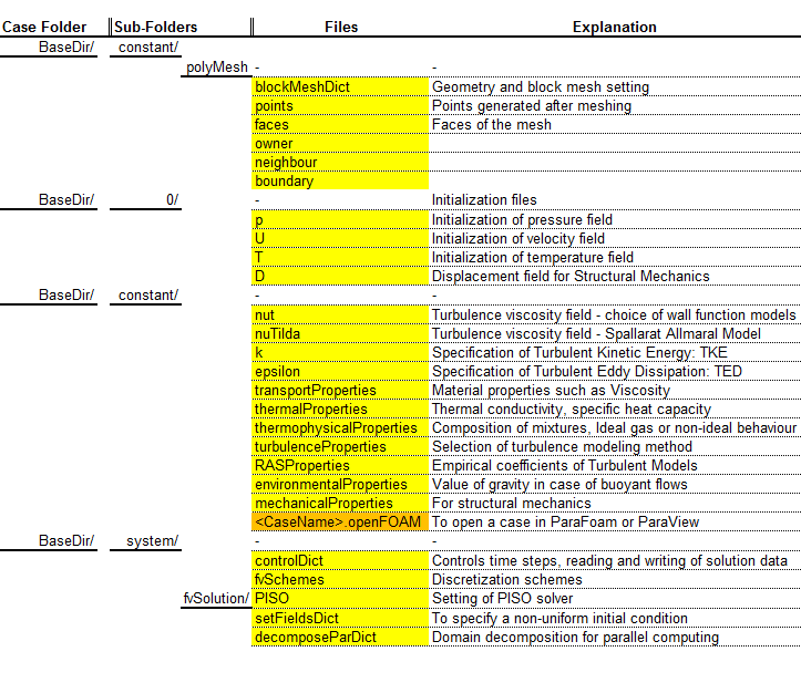
- BaseDir/system/controlDict: the system directory contains information about run-time control and solver numerics (such as discretization scheme, multi-grid solver type, relaxation factors ...)
- BaseDir/constant/polyMesh: This directory contains information about polyhedral mesh using 5 sub-dictionaries described below.
- BaseDir/constant/polyMesh/points or points.gz
- BaseDir/constant/polyMesh/faces or faces.gz
- BaseDir/constant/polyMesh/owner or owner.gz
- BaseDir/constant/polyMesh/neighbour or neighbour.gz
- BaseDir/constant/polyMesh/boundary or boundary.gz: contains information about name and type of the surface patches. Patch name defined in this file should match with patch names (boundary names) used in field variables dictionaries inside ${FOAM_CASE}/0/ folder.
- BaseDir/0/p
- BaseDir/0/U
- FOAM_CASE refers to the complete folder path of current case and can be access using $ macro substitution. For example: to include a dictionary boundaryConditions, use: #include "${FOAM_CASE}/constant/boundaryConditions" where ${FOAM_CASE} refers to the absolute path of the case folder. $WM_PROJECT_USER_DIR refers to user directory where OpenFAOM case files are stored.
- Key short-cuts to installation folders are: $FOAM_SOLVER (list of categorised solvers such as icoFoam, simpleFoam, $FOAM_UTILITIES (utilities such as blockMesh, chechMesh, postProcess...), $FOAM_SRC (source codes for entire OpenFOAM program), $FOAM_TUTORIALS (tutorial cases supplied with installation), $FOAM_RUN (user folder). OpenFOAM provides following aliases: foam='cd $WM_PROJECT_DIR', run='cd $FOAM_RUN', tut='cd $FOAM_TUTORIALS', app='cd $FOAM_APP', src='cd $FOAM_SRC'
- Folders containing executables: $FOAM_APPBIN (list of all executables and dll files), $FOAM_USER_APPBIN (folder to keep new executables created by users), $FOAM_LIBBIN (library for binaries).
- In you are using Ubuntu on Windows 10, use the command cd /mnt/f/OF to move into the folder OF on Windows drive F:/
- tree -d -L 2 $FOAM_TUTORIALS: get a list of solvers for which there are tutorial cases available. It will require command 'tree' to be installed in your OS.
- find $WM_PROJECT_DIR -name \*Dict | grep -v blockMeshDict | grep -v controlDict: get a list of utilities that use a dictionary
- The following example provides a description of the boundary condition and lists cases that use the symmetryPlane condition: foamInfo -a symmetryPlane or foamInfo totalPressure
- The boundary conditions for scalar fields and vector fields, respectively, can be listed for a given solver, e.g. simpleFoam, as follows: simpleFoam -listScalarBCs -listVectorBCs
- BaseDir/Allrun: This file describes all the things that need to be executed in order to run a case. $WM_PROJECT_DIR/bin/tools/RunFunctions, getApplication reads name of the solver from file controlDict, runApplication blockMesh runs 'blockMesh'. Watch youtube.com/watch?v=u7SSVurFhTY for more information.
- BaseDir/Allclean: Keeps file required for future re-use. All other files are deleted.
- controlDict: Excerpts from user guide: "Input data relating to the control of time and reading and writing of the solution data are read in from the controlDict dictionary. The user should view this file; as a case control file, it is located in the system directory."
- blockMeshDict: the file describing the geometry (and not the mesh, 'blockMesh' is the utility or command that creates the mesh from this geometry). This operation, 'blockmesh' creates the 5 files described below.
- points or pints.gz: the file containing node numbers and locations (X, Y, Z coordinates)
- faces or faces.gz: the file containing the face connectivity of the "points" or nodes defined in points file
- owner or owner.gz: the file containing the collection of faces which make up an 3D element
- neighbour or neighbour.gz: the file containing connectivity between the faces (each internal faces have an owner and neighbour, apart from boundary faces who have owner only). Note that it uses '..ou..' in neighbour.
- .../0/p and .../0/U are boundary condition setting and flow field initialization files. Be careful with the units! In OpenFOAM incompressible solvers, the solved pressure is plocal / ρ. Hence, unit in p dictionary should be m2/s2 i.e. [0 2 -2 0 0 0 0] and not kg/m-s2 i.e. [1 -1 -2 0 0 0 0].
- system/fvSchemes: This dictionary in the system directory sets the numerical schemes for terms, such as derivatives equations, that appear in applications being run.
- U / p / T dictionaries : boundary names can be combined using "(boundary-1 | boundary-2 | ...)". Note that there should not be any space before and after separator "|". Refer to tutorial case simpleFoam/simpleCar. E.g.
"(left|right)" { type zeroGradient; } - ".*" - match everything, "U.*" - match everything that starts with U, "(U|k|h)" - match for U, k and h, "(U|k|h)Final" - match for UFinal, kFinal, hFinal. "[a-zA-Z]*\.solve\(" matches 0 or more of the characters in the brackets, so here any letter. For instance, this would match "UEqn" or "pEqn" or "rhoEqn", the second part "\.solve\(" matches the part following the first part and simply translates to ".solve(". Thus, it will match "UEqn.solve(". "[a-zA-Z]+" would match at least one or more of the characters in the brackets.
- DT: diffusivity which resides in transportProperties dictionary, phi is a flux scalar field = U.Sf where Sf is the area of the cell faces. Thus, phi represent face fluxes.
- There are two different algorithms to solve Navier-Stokes equations. SIMPLE (simpleFoam...) - only steady state solution [pseudo-transient] and PISO (icoFoam, pisoFoam...) - both transient and steady state solution.

Step-by-step Guide for OpenFOAM simulations
Generation of computational geometry and mesh is one of the most time consuming activity. A comparison between pre-processing activity used in OpenFOAM simulation process and any other commercial program with fully-developed GUI is summarized below.| Step-1 | Commercial Program | OpenFOAM |
| Pre-processing | Geometry creation in CAD, import into CFD simulation program as IGES, STEP, PARASOLID | Create geometry inside OpenFOAM using blockMesh utility, create geometry in any 3D CAD environment, import geometry in STL for meshing using snappyHexMesh (sHM) utility. sHM requires other utilities such as surfaceCheck which can check the input STL geometry and prints overall size (bounding box) of the geometry. |
| Mesh generation in a meshing program such as ICEM CFD, ANSA, GridPro, PointWise and import into a solver dependent format such as *.msh, *.cfx5, *.ccm | Generate mesh using blockMesh, generate mesh in any other program (GMSH) and use converter utilities such as gmsh2foam, fluentMeshToFoam | |
| Naming of zone for easy selection and application of boundary condition is done in mesh generation environment | The method is equally applicable to OpenFOAM as boundary condition needs to be applied on a set of contiguous faces. |
Reading surface from "constant/triSurface/Fan_in_Duct.stl" ...
Statistics:
Triangles    : 23474
Vertices     : 11749
Bounding Box : (-550 -185 -185) (540 185 185)

Region  Size
------  ----
patch0  23474

Surface has no illegal triangles.

Triangle quality (equilateral=1, collapsed=0):
    0.00 .. 0.05  : 0.1744
    0.05 .. 0.10  : 0.1612
    ...

    min 4.76e-06 for triangle 19519
    max 0.999899 for triangle 11050

Edges:
    min 0.00290 for edge 352 points (-22.92 108.37 143.69)(-22.9 108.37 143.7)
    max 500.073 for edge 101 points (-550.0 152.62 104.55)(-50.0 157.29 97.39)

Checking for points less than 1e-6 of bounding box ((1090 370 370) metre) apart.
Found 0 nearby points.

Surface is not closed since not all edges connected to two faces:
    connected to one face : 24
    connected to >2 faces : 8
Conflicting face labels:48
Dumping conflicting face labels to "problemFaces"
Paste this into the input for surfaceSubset

Number of unconnected parts : 2
Splitting surface into parts ...

Writing zoning to "zone_Fan_in_Duct.vtk"...

writing part 0 size 1084 to "Fan_in_Duct_0.obj"
writing part 1 size 2239 to "Fan_in_Duct_1.obj"

Number of zones (connected area with consistent normal) : 10
More than one normal orientation.
- autoPatch: split the boundary into set of contiguous set of face elements, defined by specified feature angle. surfaceAutoPatch input.stl output.stl 150 will split the geometry with feature angle 150°. It works by grouping the cells having adjacent surface normals are at an angle less // than includedAngle as features // - 0 : selects no edges // - 180: selects all edges
- createPatch: Utility to create patches out of selected boundary faces. Source of faces can either be existing patches or from a faceSet
- transformPoints: Utility that allows a change in the geometry. Syntax: transformPoints . testCase –translate vector. E.g. transformPoints -case elbowNew -translate "(0.1 0 0)". Use "transformPoints -help" to get other capabilities such as rotate and scale the meshes.
- checkMesh: Use this utility to ensure mesh pass through the criteria set for OpenFOAM solver. User can change the default criteria using system/meshQualityDict.
- The default maximum value for orthogonality in OpenFOAM is 70°, standard threshold for aspect ratio is 1000 and threshold for skewness in OpenFOAM is 4.
- Excerpts from "Computational Fluid Dynamics in OpenFOAM - Mesh Generation and Quality by Rebecca Gullberg": ParaView can also be useful if the command "checkMesh" fails. For example, if some of the cells in the mesh cross the threshold for non-orthogonality, running the checkMech command will add these cells to a special set of cells, called nonOrthoFaces.
- By typing the command "foamToVTK - faceSet nonOrthofaces" the Visualization Toolkit (VTK) in OpenFOAM creates a VTK file. This VTK file can be opened in ParaView to visualize the "bad" cells.
- ParaView also contains a mesh quality filter that can be used to evaluate the quality of the cells by adjusting the threshold for different metrics. ParaView does not use the same mesh quality metrics as OpenFOAM, but it is a useful feature to get a general overview of the mesh quality.
- The two empty sides of a 2D mesh must have the same mesh distribution. The flattenMesh utility can sometimes fix the problem of "edges not aligned with or perpendicular to non-empty directions".
- refineHexMesh: Refines a hexahederal mesh by 2x2x2 cell splitting, autoRefineMesh: Refines cells near surfaces, renumberMesh: Renumbers the cell list to reduce the bandwidth.
Step-2: Thermophysical Models, Transport (Viscous) Model and Boundary Conditions - the definition of material properties, and selection of turbulence model are done through the files stored in folder 'constant' namely 'transportProperties' and 'turbulenceProperties'. The application of boundary conditions for velocity is done through file located in folder '0' as explained above. Thermophysical models models are concerned with energy, heat and physical properties. The transport modelling evaluates dynamic viscosity, thermal conductivity and thermal diffusivity (for internal energy and enthalpy equations). The thermodynamic models are concerned with evaluating the specific heat capacity from which other properties are derived. All models are located under $FOAM_SRC/thermophysicalModels folder.
hePsiThermo: General thermophysical model calculation based on compressibility: ψ = 1/(RT) and applicable only to gases. hRhoThermo: General thermophysical model calculation based on density (applicable to gases, liquids, solids). hSolidThermo: applicable only to solids.
- Reduce the bandwidth of the mesh using renumberMesh utility
- Use readFields utility to read data obtained from experiment or from previous simulation or mapFields - to map the coarse mesh results to the initial conditions for the fine mesh.
- mapFields <sourcecCase> -case <newCase> -sourceTime latestTime
- For non-consistent cases a system/mapFieldsDict dictionary needs to be used
- The flags '-parallelSource' and '-parallelTarget' are used if any or both of the cases are to be run in parallel modes.
- Chose B.C. type from basic category like "fixedValue, fixedGradient, mixed" or derived categories like "fixedProfile, inletOutlet: outlet condition with handling of reverse flow, swirlFlowRateInletVelocity, codedFixedValue: fixed value set by user coding" .... The list of available B.C. can be found in the user manual or at the last section of this page.
- Specify turbulence value at inlet and in the interior using dictionaries k, epsilon... k = 1.5 × U2 × I2 Where U is velocity magnitude and I is turbulence intensity which has a value of 0.001 (or 0.1%) for controlled external flows. At 10 [m/s] and I = 0.1%, k = 1.5E-4 [m2/s2], at 1 [m/s], it is 1.5E-6 [m2/s2]. From dimensional arguments, ε = Cμ0.75 × k1.5/L where Cμ is an empirical constant = 0.09 and L is the length scale of the flow. At 1 [m/s], I = 0.1% and L = 1 [mm], ε = 3.0E-7 [m2/s3]. At I = 10% [I = 0.1], ε = 3.0E-3 [m2/s3].
- OpenFOAM version 3.0 onwards, there is a pre-processing utility 'createZeroDirectory' to create a complete time '0' directory containing all necessary initial field files (u, p, T, k, epsilon...) and their values and boundary conditions set according to the solver name given in the case system/controlDict file. Turbulence fields are generated based on the settings provided in the turbulenceProperties file. Dictionary system/regionName for multi-region cases are referred when this utility is run.
- If you copied an existing case folder, you may use the utility 'changeDictionary' to change dictionary entries (such as the patch type for fields and polyMesh/boundary files). A changeDictionaryDict file will need to be created for this. Replacement entries starting with '~' will remove the entry.
- The non-Newtonian models such as Herschel-Bulkley can also be modeled by defining coefficients in 'transportProperties' dictionary'
mapFieldDict:
patchMap ( w-x1 w-x2 );
cuttingPatches ( fixedWalls );
The first line specify patches that have different names in the cases. The second line implies that the 'fixedWalls' patch is cutting through the source case.
Non-Newtonian models: Herschel-Bulkley type of material poses an initial resistance to flow. Once the level of yield stress τ0 has been exceeded, the material flows according to the stress-shear relation: τ = τ0 + μPLγn where μPL = plastic viscosity and n = shear rate of the material. Division of shear stress by shear rate and density of the material renders the dynamic viscosity, μ = τ / ρ γn.transportModel CrossPowerLaw; //Newtonian
CrossPowerLawCoeffs {
nu0 0.01;
nuInf 10;
m 0.4;
n 3;
}
BirdCarreauCoeffs {
nu0 1e-06;
nuInf 1e-06;
k 0;
n 1;
}
transportModel HerschelBulkley;
HerschelBulkleyCoeffs {
tau0 0.005;
k 0.001;
n 0.85;
nu0 1.0e5;
}
Step-3: Solver setting - files stored in folder 'system' can be used to select a solver, specify convergence criteria, chose relaxation factor, time steps for pseudo-transient or physically transient simulations. Rotating domains can be set using dictionary 'MRFproperties' or 'SRFProperties' under 'constant' directory. There is an attempt to consolidate the solvers and the dynamic-mesh versions such as pimpleDyMFoam, interDyMFoam are being merged to their parent solvers such as pimpleFoam and interFoam in this case.
- Use setFields (requires setFieldsDict) utility to initialize different value in various zones. This utility is very flexible, one can even read STL files (surfaceToCell) and use them to initialize fields. To implement special initials conditions, there are 3 options: use codeStream, use high level programming and/or use an external library (e.g. swak4foam - an external library that is not officially supported by the OpenFOAM foundation).
- Use utility system/decomposePar to partition the mesh for parallel processing.
- Set monitor points: for example to write average temperature to the terminal during simulation add following lines of code in system/ controlDict:
functions( avgT { functionObjectLibs ("libutilityFunctionObjects.so"); type coded; redirectType average; outputControl outputTime; code #{ const volScalarField& T = mesh().lookupObject("T"); Info<<"T avg:" << average(T) << endl; #}; } ); - Control write intervals: the intervals to write output can be controlled through controlDict file. In order to determine write interval during run time, use following code inside the controlDict dictionary:
startTime 0; endTime 100; n 5; ... writeInterval #codeStream { code #{ label dt = ($endTime - $startTime); label i = $n; os << (dt / i); #}; }; - 'foamJob' utility can be used to run an OpenFOAM job in background and redirects the output to 'log' in the case directory. foamLog - extracts xy files from OpenFOAM logs. The default is to extract for all the 'Solved for' variables the initial residual, the final residual and the number of iterations. "foamLog -l" lists all the possible variables without extracting them. One can monitor the run through non-OpenFOAM utilities such as PyFOAM.
- To terminate the execution at any time without saving the data for current iteration (time-step), press control-c. If you want to save the current iteration also, edit the controlDict file by to "runTimeModifiable yes;" if required and then add the keyword "stopAt writeNow;". Other options to 'writeNow' are nextWrite, writeNow, noWriteNow, endTime.
- Use sampleDict to create a sampling of solution over a line or a surface for subsequent post-processing.
- Graphical representation of the residuals for monitoring: The foamLog utility is script developed using commands 'grep', 'awk' and 'sed' to extract appropriate values from a log file. The source code can be located as $WM_PROJECT_DIR/bin/foamLog. It uses a database foamLog.db to know what to extract. foamLog is executed by command "foamLog log". The graphical representation can be generated by gnuplot command: set logscale y, plot "Ux_0", "Uy_0", "Uz_0", "p_0". Alternatively, pyFoam can be used to achieve same result. Command "foamLog -h" yields following description: The default is to extract the initial residual, the final residual and the number of iterations for all 'Solved for' variables. Additionally, a (user editable) database is used to extract data for standard non-solved for variables like Courant number and execution time.
foamMonitor: Monitor data with Gnuplot from time-value(s) graphs written by OpenFOAM e.g. by functionObjects. This utility requires gnuplot. Example: foamMonitor -l postProcessing/residuals/0/residuals.dat
functions  {
  #include "minMax"  // Print stats
}
where the minMax file (dictionary) contains:
minMax {
  type            fieldMinMax;  // Type of functionObject
  // Where to load it from (if not already in solver)
  libs            ("libfieldFunctionObjects.so");
  log             true; // Log to output (default: false)
  fields  (             // Fields to be monitored - runTime modifiable
    U  p
  );
}
Step-4: Post-processing - ParaView is a native post-processor for OpenFOAM result. Create a file foam.foam in the case folder and read it in ParaView. All the necessary result files will get loaded. Alternatively, use conversion utilities such as foamMeshToFluent and foamDataToFluent to post-process the result in other commercial programs. Use utility postProcess to generate intermediate outputs from OpenFOAM for subsequent post-processing in GNUPlot or ParaView: e.g. postProcess -func sampleDict -latestTime.
Refer in the later sections of this page on dictionaries requires for postProcess utility. All the available utilities can be found in applications/ utilities/ postProcessing/. Just type the command 'app' which will take you to the folder 'applications'.
The list can also be generated by the command 'postProcess -list'. Use the -help flag for more information, as usual for any other application. Examples can be found in folder $WM_PROJECT_DIR/ etc/ caseDicts/ postProcessing.
Sometimes command "postProcess -func wallShearStress -latestTime" shall give following error.--> FOAM FATAL ERROR:
Unable to find turbulence model in the database
From function virtual bool Foam::functionObjects::wallShearStress::execute()
in file wallShearStress/wallShearStress.C at line 200.
Command "postProcess -func yPlus -latestTime" shall give following error.
--> FOAM FATAL ERROR:
Unable to find turbulence model in the database

    From function virtual bool Foam::functionObjects::yPlus::execute()
    in file yPlus/yPlus.C at line 176.
"rhoSimpleFoam -postProcess -func wallShearStress" shall yield following results.
Time = 50
Reading thermophysical properties

Selecting thermodynamics package
{
    type            hePsiThermo;
    mixture         pureMixture;
    transport       const;
    thermo          hConst;
    equationOfState perfectGas;
    specie          specie;
    energy          sensibleInternalEnergy;
}

Reading field U

Reading/calculating face flux field phi

pressureControl
    pMax 205740.4
    pMin 10000

Creating turbulence model

Selecting turbulence model type RAS
Selecting RAS turbulence model kOmegaSST
Selecting patchDistMethod meshWave
RAS
{
    RASModel        kOmegaSST;
    turbulence      on;
    printCoeffs     on;
    alphaK1         0.85;
    alphaK2         1;
    alphaOmega1     0.5;
    alphaOmega2     0.856;
    gamma1          0.55555556;
    gamma2          0.44;
    beta1           0.075;
    beta2           0.0828;
    betaStar        0.09;
    a1              0.31;
    b1              1;
    c1              10;
    F3              false;
}

No MRF models present

Creating finite volume options from "system/fvOptions"

Selecting finite volume options model type limitTemperature
    Source: limitT
    - selecting all cells
    - selected 16000 cell(s) with volume 2.0996568
wallShearStress wallShearStress:
    processing all wall patches

wallShearStress wallShearStress write:
    writing object wallShearStress
    min/max(aerofoil) = (-8.64 -0.0 -3.32), (-0.751 0.0 3.32)
"rhoSimpleFoam -postProcess -func wallShearStress -latestTime" shall calculate the wall shear stress only at the latestTime step.
Function objects to derive additional data both during and after calculations, typically in the form of additional logging to the screen, or generating text, image and field files. This eliminates the need to store all run-time generated data, hence saving considerable resources. Furthermore, function objects are readily applied to batch-driven processes, improving reliability by standardising the sequence of operations and reducing the amount of manual interaction. Data derived from function objects are written to the case 'postProcessing' directory, typically in a subdirectory with the same name as the object. E.g. $FOAM_CASE/ postProcessing/ 'functionObjectName'/ 'time'/ 'data'. The function objects are options that are run time selectable. The results generated by function objects can be both obtained in the due course of simulation and after the calculation. Source codes can be found in $FOAM_SRC/ OpenFOAM/ db/ functionObjects and $FOAM_SRC/ functionObjects.
- When specified without additional arguments, the postProcess utility executes all objects defined in the controlDict: postProcess. Some functions can be invoked directly without the need to specify the input dictionary using the -func option e.g. to execute the Courant number function object: postProcess -func 'CourantNo'.
- simpleFoam -postProcess -func yPlus: write yPlus values on the walls. It creates a file named yPlus in each time directory and can be used to create contour plots in ParaView. simpleFoam -postProcess will execute all function objects defined in the controlDict.
- postProcess –func vorticity –noZero: compute and write the vorticity field for all the saved solutions excluding 0. The –noZero option means do not compute the vorticity field for the directory 0. Do not use '–noZero' option to compute and write the vorticity field for '0' time-step.
- postprocess –func 'grad(U)' –endTime: compute and write the velocity gradient or grad(U) in the whole domain (including at the walls). The –endTime option instructs to compute the velocity gradient only for the last time-step of the solution. Similarly, postprocess –func 'grad(p)' and postProcess -func 'div(T)' can be used to compute and write the divergence of the pressure and temperature fields respectively for all time steps.
- wallGradU: calculates the velocity gradient at each wall boundary.
- pisoFoam -postProcess -func CourantNo: compute and write the Courant number.
- pisoFoam -postProcess -func wallShearStress: compute and write the wall shear stresses at the walls. Since no arguments are given, it will save the wall shear stresses for all time steps in '0' directory.
- postProcess -func writeCellCentres -time tx: writes coordinates of the cell centroids to files at a given time step 'tx' as volScalarField
- Some other utilities related to extract quantitative information such as area-average values are:
- gSum: command to sum up values, similar to a "sum" in MS-Excel
- mesh.magSf(): surface area of each face of each cell present in the mesh
- mesh.magSf().boundaryField()[myPatch]: surface area of each face present in patch "myPatch"
- totalArea = gSum( mesh.magSf().boundaryField()[myPatch] ): total surface area of a patch
Few examples from "Evoking existing function objects and creating new user-defined function objects for Post-Processing" by Sankar Raju N.
Calculate y+ of the specific walls.
yPls {
 type yPlus;
 libs ("libfieldFunctionObjects.so");
 patches (leftWall rightWall stepWall);
}
Compute stress tensor parameter 'R'. One can additionally compute eddy kinematic viscosity (nut), effective kinematic viscosity (nuEff), deviatoric stress tensor (devReff), eddy dynamic viscosity (mut), effective dynamic viscosity (muEff), thermal eddy diffusivity (alphat), effective eddy thermal diffusivity (alphaEff), deviatoric stress tensor (devRhoReff).
 turbFieldsR {
 type turbulenceFields;
 libs ("libfieldFunctionObjects.so");
 field R;
}
Function object Q-criterion calculates and outputs the second invariant of the velocity gradient tensor [1/s2]. Q iso-surfaces are good indicators of turbulent flow structures. In the example below, result is displayed with the name usrQ.
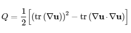
QCrit {
 type Q;
 libs ("libfieldFunctionObjects.so");
 field U;
 result usrQ;
}
To find all of the examples of Function Objects being used in the standard OpenFOAM tutorials, run the following command to get a list of tutorial cases that used them: find $FOAM_TUTORIALS -name controlDict | xargs grep 'functions' -sl
Note: All the incompressible solvers implemented in OpenFOAM namely icoFoam, simpleFoam, pisoFoam and pimpleFoam use "specific energy [J/kg] or modified pressure P = p/ρ [J/kg] where p is actual static pressure in [Pa]. Hence, during post-processing the results need to be multiplied by the density to get the pressure in [Pa].
The structure or hierarchy of the files and dictionaries used in OpenFOAM case is shown below:
Similarly, constant/combustionProperties dictionary contains settings for the combustion calculations such as combustion model parameters, fuel properties and ignition parameters (ignition time, location, duration and strength).
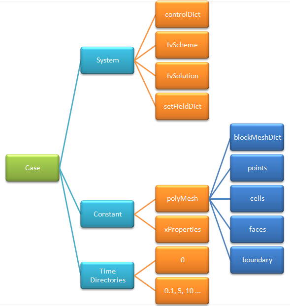
fvSolution               <-- Dictionary file
  solvers {              <-- Dictionaries
  p	{                <-- Sub-Dictionaries or Keywords
    solver PCG;
    preconditioner DIC;  <-- Values assigned to Keywords
    tolerance 1e-06;     <-- Values assigned to Keywords
    relTol 0;
 }
Most of the applications in OpenFOAM requires instruction from a plain text file called dictionaries. These are equivalent command line operation to the GUI features available in commercial software. Though, most of the dictionaries are commented well, the learning curve might still be steep for most of the beginners.
Headers of the dictionaries convey information about class and object (note that OpenFOAM has been written in C++ which is an object-oriented programming language). For example:
FoamFile {
    version     2.0;
    format      ascii;
    class       volVectorField; //dictionary, volScalarField, volTensorField
    object      U;              //p, T, gradU, sigma, k, epsilon, nut, omega, caseProperties, caseSummary
                                //controlDict, sampleDict, fvSchemes, fvSolution, transportProperties ...
}
In the example above, object 'U is of class type 'volVectorField' and should always be specified / initialized as vector such as "internalField uniform (0 0 0);". Similarly, an object of class type 'volTensorField' will need to be specified as 3×3 matrix.
A dictionary in OpenFOAM can contain multiple data entries as well as many sub-dictionaries. For a dictionary entry, the name is followed by the keyword entries in curly braces '{'. E.g.
solvers  {               //Dictionary 'solver'
  p {                    //Sub-dictionary 'p' as it is nested inside dictionary 'solver'
    solver         PCG;
    preconditioner DIC;
    tolerance      1e-06;
    relTol         0;
  }
}
Macro expansion can be used to duplicate and access variables in dictionaries. For example:
$p;                //Create a copy of dictionary 'p'
$p.tolerance;      //Access variable 'tolerance' in the dictionary 'p'
Another example of dictionary nested inside a dictionary:
boundaryField {    //Dictionary 'boundaryField'
  inlet   {        //Sub-dictionary 'inlet' as it is nested inside dictionary 'boundaryField'
    type            zeroGradient;
  }
  outlet     {     //Sub-dictionary 'outlet' as it is nested inside dictionary 'boundaryField'
    type            fixedValue;
    value           uniform 0;
  }
}
Lists or list entries on the other hand are followed by parentheses '(' for example:
vertices (         //Name of the the 'list'
  (0 0 5)
  (0 5 5)
)
Example 'blockMeshDict' files and mesh generated in OpenFOAM
The mesh generated by blockMeshDict file available with OpenFOAM distribution. 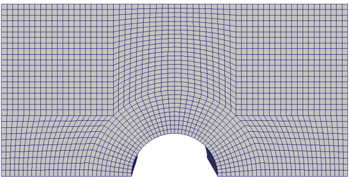
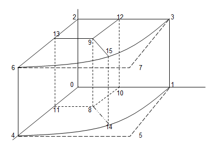
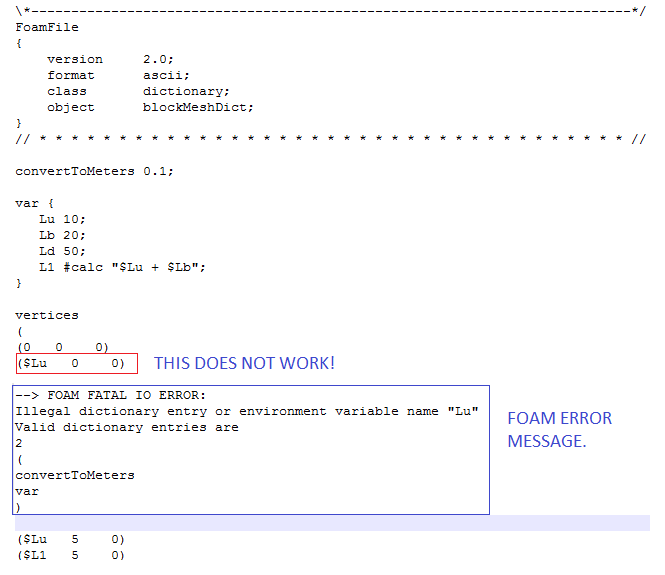
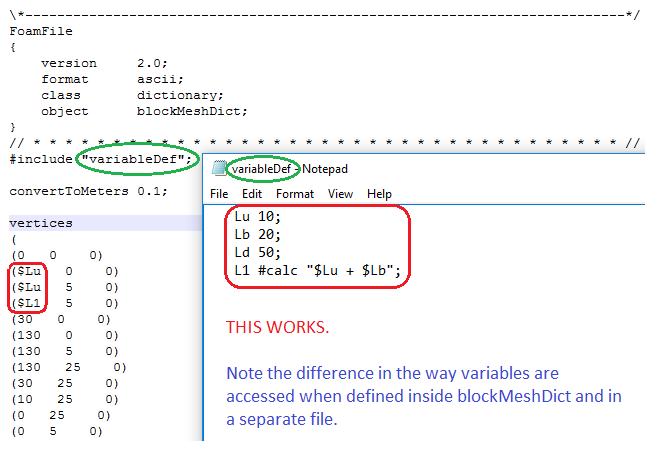
Variables or Parametric blockMeshDict
It is possible to use variables or parameters to define meshing features in blockMeshDict. If #calc function is used, blockMesh creates a runtime folder dynamicCode (first run of blockMesh) in the case folder. Refer to the screenshots for sample use of variables in blockMeshDict and what works and what does not [tested in Version: v1606+ on Microsoft Windows 10].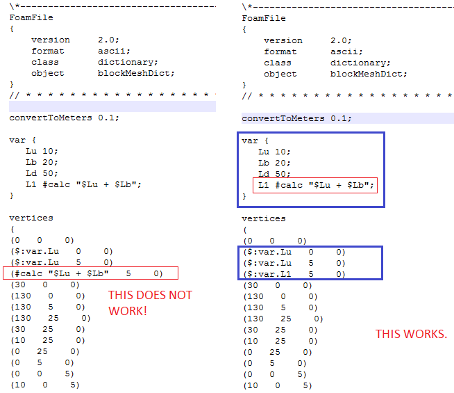
  flowVelocity         (10 0 0);
  pressure             10000;
  turbulentKE          0.1;
  turbulentOmega       0.3;
  #inputMode           merge
This file has been included in 'U' dictionary as
  #include        "initConditions"
  dimensions      [0 1 -1 0 0 0 0];
  internalField   uniform $flowVelocity;
Other example of 'include' directive for definition of variables in blockMeshDict is explained below.
Variables can be accessed within different levels of sub-dictionaries, or scope. Scoping is performed using a ‘. ’ (dot) syntax, illustrated by the following example, where b is set to the value of a, specified in a sub-dictionary called subdict.
subdict  {
  a 10;
}
b $subdict.a;
There are further syntax rules for macro expansions: to traverse up one level of sub-dictionary, use the '.. ' (double-dot) prefix, to traverse up two levels use '... ' (triple-dot) prefix, to traverse to the top level dictionary use the ':' (colon) prefix (most useful), for multiple levels of macro substitution, each specified with the '$' dollar syntax, '{}' brackets are required to protect the expansion.
a 10; b a; c ${${b}}; // returns 10, since $b returns "a", and $a returns 10
dict1 {
  b $..a; // double-dot takes scope up 1 level, then "a" is available
  subdict2 {
    c $:a; // colon takes scope to top level, then "a" is available
  }
}
Dirichlet B.C. – prescribes the value of the dependent variable on the boundary and is specified with keyword "fixedValue" in OpenFOAM. Neumann B.C.- prescribes the gradient of the variable normal to the boundary and is specified with keyword "fixedGradient or zeroGradient" in OpenFOAM. In OpenFOAM, boundary fields are calculated as per following equation where "refValue", φREF and "refGrad" are the value and the gradient taken as reference values. Here f is a fraction that switches the boundary condition between a Dirichlet BC (f = 1) and a Neumann BC (f = 0). δ is the center patch face to center cell distance and φi is the field variable at cell center.
φB = f × φREF + (1 - f) × (φi + refGrad × δ)
The recommended use of variables to define the boundary conditions can be found in folder $FOAM_SRC/ finiteVolume/ fields/ fvPatchField/ derived.Inlet Boundary Condition from Volumetric / Mass Flow Rate: This method specifies uniform velocity at inlet face. For volumetric heat flow, use the following settings.
  inletZone  {
    type                 flowRateInletVelocity;   //Calculate velocity field from volumetric flow rate
    volumetricFlowRate   1.0;                     //volume flow rate in [m3/s]
    value   uniform      (1 0 0);                 //Initial value: does not affect the B.C.
  }
To calculate velocity from mass flow rate, the solver needs to know the density. Hence, DataEntry type 'rho' needs to be specified in this case.
  inletZone  {
    type                 flowRateInletVelocity;   //Calculate velocity field from volumetric flow rate
    massFlowRate         1.0;                     //volume flow rate in [m3/s]
    rho                  rho;                     //Name of density field
    rhoInlet             1.185;                   //Density at inlet in [kg/m3]
  }
Boundary conditions in cylindrical coordinate system
  inletZone  {
    type            cylindricalInletVelocity;    //specify that it is in cyl CS.
    axis            (0 1 0);                     //z-axis of cylindrical CS
    centre          (1 0 0);                     //centre of CS w.r.t global CS
    axialVelocity   constant  10;                //velocity along axial direction
    radialVelocity  constant -5;
    rpm constant    1000;
  }
Boundary conditions: Total Pressure - phi used in the dictionary totalPressure below is a flux scalar field = U.Sf where Sf is the area vector of the cell faces and U is velocity field obtained by interpolating velocities at cell centers. mesh.Sf() creates a vector field - surface normal for each surface of the mesh. phi field is calculated by dot product: linearInterpolate(U) & mesh.Sf where '&' denotes the dot product of two vectors.
  outletZone  {
    type   totalPressure;
    U      U;
    phi    phi;                        //Name of flux field
    rho    rho;                        //Name of density field
    psi    none;                       //1/R/T: R = Gas constant
    gamma  1.4;                        //Adiabatic exponent = Cp / Cv
    p0     uniform 1e5;                //Total pressure value
  }
- For subsonic conditions (Ma < 0.3): p0 = p + 1/2 * ρ * U * U.
- For transonic conditions (γ ≤ 1.0) - p0 = p * [1 + 1/2 * ψ * U * U], p/RT = ρ, Thus: p0 = p + 1/2 * ρ * U * U.
- For transonic conditions (γ > 1.0) - p0 = p * [1 + (γ-1)/2 * Ma](γ-1)/γ
Boundary conditions: Parabolic Velocity Profile in Y-direction at Inlet - Excerpt from a post on cfd-online.com: "codedFixedValue boundary condition method attempts to load a shared library using case-supplied C++ code, so you need to allow your FOAM to execute user written code. You should switch "allowSystemOperations" in .../etc/controlDict from 0 to 1." The implementation of codeStream for diction 0/U is described below.
Boundary conditions codedFixedValue and codedMixed are derived from codeStream and let you access more information of the simulation database (e.g. time). Another feature of these boundary conditions, is that the code section can be read from an external dictionary (system/codeDict), which is run-time modifiable. The boundary condition codedMixed works in similar way. This boundary condition gives you access to fixed values (Dirichlet BC) and gradients (Neumann BC).
dimensions [0 1 -1 0 0 0 0];
internalField uniform 10;

inletZone {                          //options for type: codedMixed, fixedValue
  type         codedFixedValue;      //B.C. - designated by term 'Fixed'
  value        $internalField;       //Initial value or use #codeStream
  redirectType parabolicInlet;       //Unique name for this boundary patch

  // Note about initial value - it is specified so the utility always has
  // a starting value to work with (e.g. when plotting boundary values using
  // ParaView at time 0). In this case the "uniform 10" value is substituted
  // for time '0'. At later times, boundary values are evaluated by solver.

  // codeStream reads 3 entries: 'code', 'codeInclude' (optional), 'codeOptions'
  // (optional) and uses those to generate library sources inside codeStream/
  // Note the #{ ... #} syntax is a 'verbatim' input mode that allows inputting
  // strings with embedded newlines. Method to read mesh if different for the
  // internal field and boundary faces.

  code #{
    const IOdictionary& d = static_cast<const IOdictionary&> (
      dict.parent().parent()            // access current dictionary
    );

    //Access the mesh database.
    const fvMesh& mesh = refCast<const fvMesh>(d.db());

    //Specify the actual name of the patch: get the label ID
    const label zoneId = mesh.boundary().findPatchID("inletZone");

    //Access the boundary mesh information using label ID 'zoneId'
    const fvPatch& patch = mesh.boundary()[zoneId];

    //Initialize velocity components -  patch.size() = number of faces
    vectorField U(patch.size(), vector(0, 0, 0));

    //codeStream recognises regular macro substitutions using the '$' syntax

    //Create boundary condition without loop
    vector dir = vector(0, 1, 0);       //Get unit vector along x-direction
    scalarField var = patch().Cf()&dir; //& = dot product, Cf = face centre
    scalarField value = 10.0*(1.0 - pow(var, 2) / pow(0.5, 2));
    vector(1, 0, 0) * value;            //Velocity components as vector field

    const scalar pi = constant::mathematical::pi;
    V0 = 10.0;
    //Create boundary condition with loop
    forAll(U, i)  {                    //for (int i=0; patch.size()<i; i++)
      const scalar y = patch.Cf()[i][1];
      U[i] = vector($V0 * (1 - pow(var,2) / pow(0.5, 2));
    }
    U.writeEntry("", os);              //Write values of U to the dictionary
  #}

  //Optional - Files needed for compilation
  codeInclude #{
    #include "fvCFD.H"
    #include <cmath>
    #include <iostream>
  #};

  //Optional - Compilation options
  codeOptions #{
    -I$(LIB_SRC)/finiteVolume/lnInclude \
    -I$(LIB_SRC)/meshTools/lnInclude
  #};

  //Optional - Libraries needed for compilation, required only to visualize
  //the output of the boundary condition at time zero
  codeLibs #{
    -lmeshTools \
    -lfiniteVolume
  #};
}
Wildcard character: If the boundary names end with a certain suffix, wildcard characters can be used to specify boundary conditions in a compact manner. "inlet.*" matches any word beginning inlet, including inlet itself, because '.' denotes "any character" and '*' denotes "repeated any number of times, including 0 times". "(inlet|output)" matches inlet and outlet because '()' specifies an expression grouping and '|' is an OR operator.
Either                             or
"(lt|rt|bt)Wall"{                  "*Wall"{
  type fixedValue;                    type fixedValue;
  value uniform (0 0 0);              value uniform (0 0 0);
}                                  }
Boundary conditions: Fan
Fan at Inlet
inletZone  {
  type            fanPressure;    //Name of fan boundary condition
  fileName        "fanPQdata";    //Name of file containing P-Q data
  outOfBounds     clamp;          //Instruction for handling out-of-bound values
  direction       in;             //Inflow direction
  p0 uniform      0;              //Initial value only. Gets updated as per fanPQdata
  value uniform   0;
}
Fan at Outlet
outletZone  {
  type            fanPressure;    //Name of fan boundary condition
  fileName        "fanPQdata";    //Name of file containing P-Q data
  outOfBounds     clamp;          //Instruction for handling out-of-bound values
  direction       out;            //Inflow direction
  p0 uniform      0;              //Initial value only. Gets updated as per fanPQdata
  value uniform   0;
}
Non-uniform or time-dependent boundary conditions
Example: Specify a ramped velocity at inlet - U = MIN(5.0 [m/s], 0.01 * t). timeVaryingMappedFixedValue can be used to specify test data (e.g. measured values of U, k and ε). Boundary condition type 'codedFixedValue' constructs on-the-fly a new boundary condition (derived from fixedValueFvPatchField) which is then used to evaluate. A special form is if the 'code' section is not supplied. In this case the code is read from a (runTimeModifiable) dictionary system/codeDict which would have a corresponding entry:
patchName {
  code  #{
    operator==(min(10, 0.1*this->db().time().value()));
  #};
When code' section is supplied in the field dictionary 'U':
inletZone  {
  type          codedFixedValue; //Description of B.C. type
  value         uniform 0;       //Initial value
  redirectType  rampedVelcity;   //Name of new boundary condition type

  code #{
    const scalar t = this->db().time().value();  //Get time
    operator == (min(5.0, 0.01 * t));
  #};
}
Similarly boundary condition type 'codedMixed' can be used to generate Robin boundary conditions on-the-fly. This is a combination of fixed value and gradient value defined as φFACE = f * φREF + (1-f) * [φCELL + Δ(∇φREF)] where f = value fraction and Δ = distance between face and the centroid of the cell. 'codedFixedValue' and 'mixed' can be combined to get a 'codedMixed' boundary condition type on-the-fly.
inletZone {
  type            mixed;        //It tells the solver it is Robin-type B.C.
  refValue        10.0;         //Fixed component
  refGradient     2.0;          //Gradient component
  valueFraction   0.5;          //Fraction f in the above equation
}
Convective Boundary Conditions
Following setting can be applied in 'T' file.wallConvective {
type externalWallHeatFluxTemperature; //to model only convection
Ta uniform 300.0; // Reference temperature q''= h*(T-Ta)
h uniform 10.0; // HTC value [W/m^2]
value uniform 300.0; // Boundary Initialization Temperature
kappa solidThermo; // -kappa x dT/dx = h *(T - Ta)
//fluidThermo, solidThermo, lookup, directionalSolidThermo
kappaName none;
}
Axi-symmetry and Wedge Boundary Condition: Note that blockMesh will not work if wedge angle is > 15°. A tutorial example can be found in incompressible/ simpleFoam/ pipeCyclic case.
Volumetric Heat and Momentum Sources
Following setting can be applied in 'fvOption' file in the folder 'system'. Alternatively, the dictionary 'porosityProperties' can be used in 'constant' folder.Porous Domains - reference tutorial case: incompressible\ simpleFoam\ simpleCar\ system - porous media is modeled by adding a source term Si to the momentum equations. A porosity value 0 < γ < 1 is added to the time derivative. The source term is represented in the Darcy-Forchheimer law as a viscous (linear) loss term and an inertial (parabolic) loss term. The source term can also be modeled as a power-law of the velocity magnitude in the form Si = C0.|u|C1.
porousZoneX {
 type            explicitPorositySource;
 active          true;
 explicitPorositySourceCoeffs {
   type            DarcyForchheimer;
   selectionMode   cellZone;
   cellZone        porousZone;
   DarcyForchheimerCoeffs  {
    d   d [0 -2 0 0 0 0 0] (5e7 -1000 -1000);
    f   f [0 -1 0 0 0 0 0] (0 0 0);
	//A local coordinate system belonging to the porous media is created from
	//the vectors e1 and e2. The pressure loss in the local coordinate system is
	//then defined with the vectors d and f.
    coordinateSystem {
      type            cartesian;
      origin          (0 0 0);
      coordinateRotation {
       type            axesRotation;
       e1              (1 0 0);
       e2              (0 1 0);
      }
    }
   }
  }
}

//The local cylindrical coordinateSystem is specified by a coordinateRotation
//of type localAxesRotation. The user specifies: e3, the axis of rotation (z)
//of the local cylindrical coordinate system; and, the origin, from which the
//radial direction (r) is constructed by the vector from the origin to local
//cell centre.

porosityCylindrical {
  type            DarcyForchheimer;
  cellZone        porosity;

  DarcyForchheimerCoeffs {
    d   d [0 -2 0 0 0 0 0] (0 1e5 0);
    f   f [0 -1 0 0 0 0 0] (0 0 0);

    coordinateSystem {
      type    cartesian;
      origin  (0 0 0);
      coordinateRotation {
       type    localAxesRotation;
       e3      (0 0 1);
      }
    }
  }
}
// In this case, the viscous momentum sink (0 1e5 0) denotes a value of 1e5
// in the circumferential direction and zero in radial and axial directions.
volumeHeatSource {
  type        scalarSemiImplicitSource;
  active      true;
  scalarSemiImplicitSourceCoeffs {
    selectionMode   cellZone;
                    //cellZone, cellSet, points, all
                    //Domain where the source is applied
    cellZone        solidDomain;
    volumeMode      specific;  //specific | absolute
    injectionRateSuSp    {
      h (100000 0);
      /* S(T) = Su + Sp * T  ->  Su = q, Sp = 0
      q''' = 'specific' volumetric generation [W/m^3] = 100,000
      q = 'absolute' volumetric generation [W]                      */
    }
  }
}
Initialization
Initialization using a STL file with setFields:defaultFieldValues (
volScalarFieldValue alpha.water 0
);
regions (
surfaceToCell {
file "./geom/patchZone.stl";
outsidePoints ((0.50 0.75 0.00));
includeInside true;
includeOutside false;
includeCut false;
fieldValues (
volScalarFieldValue alpha.water 1
);
}
);
Solution initialization using codeStream
The code section of the codeStream IC in the body of the file alpha.water is as follows,code #{
//Access internal mesh information
const IOdictionary& d = static_cast<const IOdictionary&>(dict);
const fvMesh& mesh = refCast<const fvMesh>(d.db());
scalarField alpha(mesh.nCells(), 0.); //Initialize scalar field to zero
forAll(alpha, i) {
//Access cell centers coordinates
const scalar x = mesh.C()[i][0];
const scalar y = mesh.C()[i][1];
//Assign values to alpha
if (y >= 1.0*cos(0.5*constant::mathematical::pi*x)) {
alpha[i] = 1.;
}
}
alpha.writeEntry("", os); //Write output to input dictionary
#};
Contact Resistance
Following setting can be applied to the boundary field in 'T' file.solidZone_to_waterDomain {
//type calculated;
type compressible::turbulentTemperatureCoupledBaffleMixed;
value uniform 300;
//"value" entry is only an 'initialization' value at the interface.
Tnbr T;
kappa solidThermo;
kappaName none;
/*define thermal contact resistance between regions by giving the
thickness and the conductivity of the inter-region layers. */
thicknessLayers (1e-3); // value in [m] - Rk = [K/W] = [m] / [W/m.K]
kappaLayers (5e-4); // Value in [W/m.K]
}
Cavitation
Cavitation phenomena can be modeled using 'thermodynamicProperties' such as one described below. The theory of Schnerr-Sauer (SS) and Zwart-Gerber-Belamri (ZGB) cavitation models are implemented in OpenFOAM.barotropicCompressibilityModel linear; psiv 2.5e-06; rholSat 830; psil 5e-07; pSat 4500; rhoMin 0.001;
Data Interpolation
The results from one simulation to another can be interpolated using utility mapFields. The command "mapFields -case REFCASE -sourceTime latestTime -consistent" can be used to map data from reference simulation 'REFCASE' to the new simulation. A summary of OpenFOAM tutorials can be found on this page. This is being continuously revised and updated with additional information. The summary of tutorials on Multi-Phase flow are here.To use SIMPLEC algorithm instead of SIMPLE, add following like in fvSolution files: SIMPLE { consistent true ; }
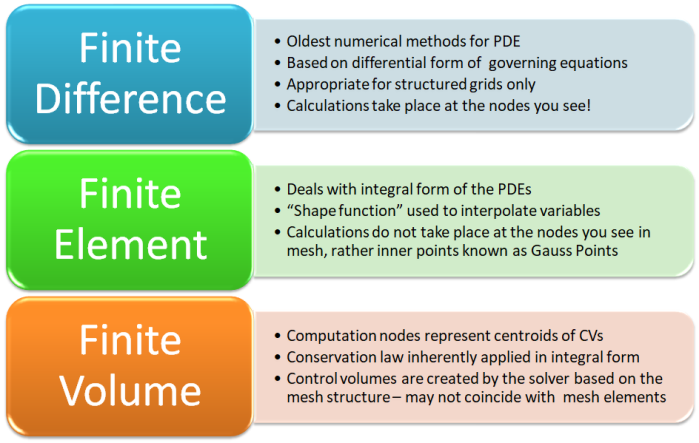
OpenFOAM by design is a Finite Volume solver (even structural problems which are dominated by Finite Element technique can be solved using OpenFOAM) and can handle any type of mesh (including the polyhedral). Following info-graphics provides a concise difference between the three numerical techniques.
6DOF Solver in OpenFOAM
Having all six degrees of freedom implies that the object can translate and rotate along all three axes in a three dimensional system. This is a generic definition and usually 2 or 3 DOF are encountered in practical situations. Usually planes may undergo all 6DOF during special manoeuvring.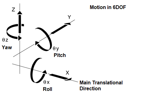
The tutorial multiphase\compressibleInterDyMFoam\laminar contains two cases (sloshingTank2D and sphereDrop) on dynamic mesh with multiphase flows.
Other utilities for moving mesh are:- moveMesh: A solver utility for moving meshes.
- moveEngineMesh: A solver utility for moving meshes for engine calculations.
- moveDynamicMesh: Move a mesh according to the motion and topological changes specified in the dictionary constant/dynamicMeshDict.
- pimpleDymFoam, interDymFoam are the solvers available for dynamic mesh (moving mesh, MRF) with and without topology changes. In recent versions (OpenFOAM v1806 or later) the dynamic mesh functionality in pimpleDyMFoam has been merged into pimpleFoam and the pimpleDyMFoam tutorials moved into the pimpleFoam tutorials directory.
Run-time Outputs
fieldFunctions
functionObjects are general libraries that can be attached run-time to the solver without having to re-compile the solver. A functionObject is added to a solver by adding a functions entry in system/controlDict dictionary. E.g. The fieldMinMax functionObject can be found in damBreakLeft/system/controlDict. Output in stored in time directory according to the time when it was initialized. Method to develop your own fieldFunction is described in this tutorial.functions {
minMaxU {
type fieldMinMax;
libs ("libfieldFunctionObjects.so");
enabled true;
log false;
write true;
fields (
U
);
mode magnitude;
writeControl timeStep;
writeInterval 1;
}
}
Post-processing Utilities and functionObjects
While the results from OpenFOAM can be post-processed both quantitatively and qualitatively in ParaView or many other post-processors, there are some postProcessing utility available inside the solver. This will help avoid the interpolation error as values inside OpenFOAM are calculated as same discretization and interpolation scheme as the solution of field variables. This feature can be accessed by adding object 'function' in 'controlDict' dictionary. Available options are - value of attribute 'type' in function examples described below. Note that this utility supersedes foamCalc utility available in older version.- fieldAverage - temporal (time) averaging of field variables such as U, p, T
- forces - this function object calculates pressure forces, viscous forces and moments
- forceCoeffs - use this function to calculate lift, drag and moment coefficients about a given centre of rotation
- isoSurface - to generate isosurface of given fields in one of the standard sample formats say VTK
- cuttingPlane - it create surface cut with one of the fields data
- streamLines - this function generates streamlines in one of the sample formats
functionObject for Pressure Drop between two zones
 deltaP {
 type         fieldValueDelta;
 functionObjectLibs ("libfieldFunctionObjects.so");
 enabled      true;
 region1 {
  writeFields off;
  type        surfaceRegion;
  regionType  patch;
  name        inlet;

  operation   sum;
  fields (
   phi
  );
 }

 region2  {
  writeFields off;
  type        surfaceRegion;
  regionType  patch;
  name        outlet;
  operation   sum;
  fields (
   phi
  );
 }
 operation    subtract;
}
functionObject for mass flow rate at a boundary patch
outletMdot  {
 type           surfaceRegion;
 functionObjectLibs ("libfieldFunctionObjects.so");
 enabled        true;

 //writeControl outputTime;
 writeControl   timeStep;
 writeInterval  1;

 log            true;
 writeFields    false;
 regionType     patch;
 name           outlet;

 operation      sum;
 fields (
  phi
 );
}
The fieldAverage functionObject calculates the time-average of specified fields and writes the results in the time directories. It needs to be added to the functions dictionary in controlDict. Example can be found in pisoFoam /les /pitzDaily case.
fieldAvgU {
  type         fieldAverage;
  libs ("libfieldFunctionObjects.so");
  enabled      true;
  writeControl outputTime;
  fields (
   U {
    mean       on;
    prime2Mean on; //RMS
    base       time;
   }
  );
}
#include "ExtFunctionObjects" can be used to include to call an external dictionary with the functionObjects definition.
postProcess -func surfaces is used to extract surfaces in VTK (ParaView) format. Dictionary file example can be located in folder $WM_PROJECT_DIR /etc /caseDicts /postProcessing /visualization /surfaces
postProcess can also be used to calculate new fields from existing ones. E.g. postProcess -func 'div(U)' -case pitzDaily
Example to calculate lift and drag coefficients are given below:
  functions {
    forces     {
        type            forceCoeffs;      //postProcessing -list: available variables
        libs            ("libforces.so");
        writeControl    timeStep;         //As multiple of timesteps
        writeInterval   1;                //Every timestep

        patches (cylWall);                //Walls to be used for force calc

        log         true;
        rhoName     rhoInf;               //Indicates incompressible
        rhoInf      1.185;                //Ref. density - not used in incompressible flows
        CofR        (0 0 0);              //Centre of Rotation
        liftDir     (0 1 0);              //Direction of list:Y-axis in this case
        dragDir     (1 0 0);              //Direction of drag: X-xis in this case
        pitchAxis   (0 0 1);              //Pitching axis: Z-axis in this case
        magUInf     50.0;                 //Reference velocity magnitude
        lRef        0.50;                 //Reference length scale
        Aref        1.00;                 //Reference area
    }
  }
CD = FD / [2 * AREF * ρINF * VINF2]. The reference length scale can be 'diameter' in case of flow over a cylinder, chord length in case of flow over an airfoil, length of the car along flow direction in case of external aerodynamics over a car. Similarly, AREF is usually D×L in case of flow over a cylinder, maximum height * maximum width in case of a car.
Similarly, to get residuals for any field variable, following 'function' object needs to be added inside 'controlDict' dictionary.
functions  {
  residuals   {
    type             residuals;      //postProcessing -list: available options
    functionObjectLibs ("libutilityFunctionObjects.so");
    enabled          true;
    outputControl    timeStep;
    outputInterval   5;              //Every 5 timestep
    fields (p U k epsilon T);
  }
}
Two other examples to write value of pressure at two 'probe' locations and average pressure of a wall surface can be found in examples multiphase / interDyMFoam / ras / sloshingTank2D / system / controlDict and incompressible / pisoFoam / pitzDaily / system / controlDict. The values can be used to plot as monitor points during and/or after the simulation.
The probes functionObject probes the development of the results during a simulation, writing to a file in the directory postProcessing/probes.
The probes function can be copied to the local system directory using "foamGet probes" and configured as per user's need. The 'singleGraph' function samples data for graph plotting. The singleGraph file should be copied using 'foamGet' into the system directory to be configured (example in pitzDaily case). It creates a folder 'singleGraph' inside folder postProcessing and saves x-y data at each time directory. The files are named as line_U.xy, line_p.xy, line_T.xy ...
functions {
 probeSolid    {                    //Name of 'probe' block
   type            probes;
   libs            ("libsampling.so");
   writeControl    writeTime;

   regions         solid;           //Only if multiple zones such as in CHT
   probeLocations  (
    (0  9.95 19.77)
    (0 -9.95 19.77)
   );
   fixedLocations  false;
   fields(
     p Ux
   );
 }
 //When solver is run, time-value data is written into p files in postProcessing/probes/0.

 probeFluid {
  type            probes;
  libs            ("libsampling.so");
  writeControl    writeTime;
  //enabled true;
  //writeControl  timeStep;
  //writeInterval 1;
  region          fluid;          //Only if multiple zones such as in CHT
  probeLocations  (
    (0  5.55 5.555)
    (0 -5.55 5.555)
  );
  fixedLocations  false;
  fields (
   p U T Ux Uy Uz
  );
 }

 wallPressure   {
   type            surfaces;      //On surfaces defined below
   libs            ("libsampling.so");
   writeControl    writeTime;
   surfaceFormat   raw;
   fields          (p);
   interpolationScheme cellPoint;

   surfaces (
    walls   {
     type        patch;
     patches     (walls);
     triangulate false;
   }
  );
 }
}
Content inside the dictionary 'system/singleGraph'.
singleGraph {
  start   (0.0 0.0 0.0);
  end     (0.1 0.0 0.0);
  fields  (p U T);

  #includeEtc "caseDicts/postProcessing/graphs/sampleDict.cfg"
  //Some installation does not recognize the caseDicts path
  //Use "${WM_PROJECT_DIR}/etc/caseDicts/postProcessing/graphs/sampleDict.cfg"
  setConfig {
    axis    distance;
    //axis  y;
  }

  // Must be last entry
  #includeEtc "caseDicts/postProcessing/graphs/graph.cfg"
  //"${WM_PROJECT_DIR}/etc/caseDicts/postProcessing/graphs/graph.cfg"
}
The variables p, U and T are extracted along a horizontal line at 100 points and the results are written in <case folder> /postProcessing /singleGraph.
The formatting of the graph is specified in configuration files in $FOAM_ETC /caseDicts /postProcessing /graphs. The sampleDict.cfg file in that directory contains a setConfig sub-dictionary.
'axis' specifies how to write point coordinates. The options are:- x or y or z: x or y or z coordinate only
- xyz: three columns
- distance: distance from start of sampling line (if uses line) or distance from first specified sampling point
sampleDict
The sampleDict file contains a sets sub-dictionary which defines where the fields should be sampled:
sets (
 line { // name of the set
   type uniform; // type of the set
   axis x;
   start (-0.05 0 0);
   end   ( 0.10 0 0);
   nPoints 1000;  //nPoints number of sampling points for uniform - default is 100
 }
);
sets functionObject: This functionObject is used to sample field data on a line. The output of this functionObject is saved in ASCII format in the files line1_p.xy and line1_U.xy located in the time directories inside the folder postProcessing/setsDataOnLine. Here line1 in line1_p.xy is the name of the sets.
setsDataOnLine {
 type         sets;
 functionObjectLibs ("libfieldFunctionObjects.so");
 enabled      true;
 writeControl outputTime;
 interpolationScheme cellPointFace;
 setFormat    raw;
 sets (
  line1 {
    type      midPointAndFace;
    axis      x;
    start     (-0.002 -0.002 0.20);
    end       ( 0.002  0.002 0.20);
  }
 );

 fields (
   U
   p
 );
}
The sampleDict contains entries to be set according to the user needs. The choice for the interpolationScheme can be one of the following. Vertex values are determined from neighboring cell-centre values whereas face values determined using the current face interpolation scheme for the field (linear, gamma ...).
interpolationScheme cellPoint;- cell : use cell-centre value only, constant over cells, no interpolation at all
- cellPoint : use cell-centre and vertex values
- cellPointFace : use cell-centre, vertex and face values
- uniform: evenly distributed points on line
- face: one point per face intersection
- midPoint: one point per cell, in between two face intersections
- midPointAndFace: combination of face and midPoint
- curve: specified points, not necessary on line, uses tracking
- cloud: specified points, uses findCell
Cutting Planes: postProcess -func surfaces is used to extract surfaces in VTK (ParaView) format. Dictionary file example can be located in folder $WM_PROJECT_DIR /etc /caseDicts /postProcessing /visualization /surfaces. Example dictionary:
#includeEtc "caseDicts/postProcessing/visualization/surfaces.cfg"
fields (p U);
surfaces (
 zNormal {
  $cuttingPlane;
  pointAndNormalDict  {
   basePoint (0.05 0.05 0.005); // Overrides default basePoint (0 0 0)
   normalVector $z; // $y: macro for (0 0 1)
  }
 }
 p0 {
  $isosurface;
  isoField p;
  isoValue 0;
 }
 movingWall {
  $patchSurface;
  patches (movingWall);
 }
);
More examples are:
functions {
  cuttingPlane {
    type                surfaces;
    functionObjectLibs  ("libsampling.so");
    outputControl       outputTime;
    surfaceFormat       vtk;
    fields              (U p T);
    interpolationScheme cellPoint;
    surfaces (
      yNormal {
        type            cuttingPlane;
        planeType       pointAndNormal;
        pointAndNormalDict {
          basePoint     (0.1 0.0 0.0);
          normalVector  (1.0 0.0 0.0);
        }
        interpolate true;
      }
    );
  }
}
Streamlines
functions {
  streamLines {
    type          streamLine;
    outputControl outputTime;
    setFormat     vtk;     //Options: gnuplot, xmgr, raw, jplot, csv, ensight
    UName         U;
    trackForward  true;
    fields        (p U);   //Streamlines can be coloured by scale of pressure
    lifeTime      1000;
    nSubCycle     5;
    cloudName     particleTracks;
    seedSampleSet uniform; //Options: cloud, triSurfaceMeshPointSet
    uniformCoeffs {
      type        uniform;
      axis        x;       //Option: distance
      start       (0 0 0);
      end         (5 0 0);
      nPoints     20;
    }
  }
}
sampling
The runtime sampling of data on a line or surface ... can be done using sample utility along with sampleDict dictionary. An example of sampleDict dictionary with all relevant comment can be found here.Plots can also be generated with Python and Matplotlib. Example code (reference: Examples of how to use some utilities and functionObjects by Hakan Nilsson, Chalmers / Applied Mechanics / Fluid Dynamics) is given below. Type python plotPressure.py at the command prompt.
#!/usr/bin/env python
description = """ Plot the pressure samples"""
import os, sys
import math
from pylab import *
from numpy import loadtxt
def addToPlots( timeName ):
	fileName = "cavity/postProcessing/singleGraph/" + timeName + "/line_p.xy"
	i=[]
	time=[]
	abc =loadtxt(fileName, skiprows=4)
	for z in abc:
		time.append(z[0])
		i.append(z[1])
	legend = "Pressure at " + timeName
	plot(time,i,label="Time " + timeName )

	figure(1);
ylabel(" p/rho "); xlabel(" Distance (m) "); title(" Pressure along sample line ")
grid()
hold(True)
for dirStr in os.listdir("cavity/postProcessing/singleGraph/"):
	addToPlots( dirStr )
legend(loc="upper left")
savefig("myPlot.jpeg")
show() #Problems with ssh
Disclaimer:
This content is not approved or endorsed by OpenCFD Limited, the producer of the OpenFOAM software and owner of the OpenFOAM and OpenCFD trademarks.Some historical facts:
- FOAM was originally written by Henry Weller et al. at Imperial College of London (interestingly, many CFD applications have genesis associated with this academy), which was initially sold as commercial code by company named Nabla Limited. In 2004, it was renamed to OpenFOAM while releasing under GNU Public License.
- FoamX was dropped from OpenFOAM V1.5 onwards. FoamX was a GUI that can manage cases on a local machine as well as over a distributed network.
- Excerpts from: "OpenFOAM for Computational Fluid Dynamics - Goong Chen, Qingang Xiong, Philip J. Morris, Eric G. Paterson, Alexey Sergeev, and Yi-Ching Wang" -- OpenFOAM was born in the strong British tradition of fluid dynamics research, specifically at The Imperial College, London, which has been a center of CFD research since the 1960s. The original development of OpenFOAM was begun by Prof. David Gosman and Dr. Radd Issa, with principal developers Henry Weller and Dr. Hrvoje Jasak. It was based on the finite volume method (FVM), an idea to use C++and object-oriented programming to develop a syntactical model of equation mimicking and scalar-vector-tensor operations. A large number of Ph.D. students and their theses have contributed to the project. Weller and Jasak founded the company Nabla Ltd, but it was not successful in marketing its product, FOAM (the predecessor of OpenFOAM), and folded in 2004. Weller founded OpenCFD Ltd. in 2004 and released the GNU general public license of OpenFOAM software. OpenFOAM constitutes a C++ CFD toolbox for customized numerical solvers (over sixty of them) that can perform simulations of basic CFD, combustion, turbulence modeling, electromagnetics, heat transfer, multiphase flow, stress analysis, and even financial mathematics modeled by the Black-Scholes equation. In August 2011, OpenCFD was acquired by Silicon Graphics International (SGI). In September 2012, SGI sold OpenCFD Ltd to the ESI Group. --
More examples of blockMeshDict
This is a parametric version of a simple diffuser with rectangular cross-section - blockMeshDict for diffuser.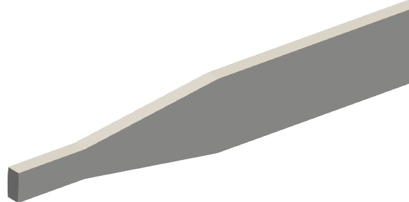
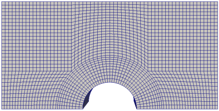
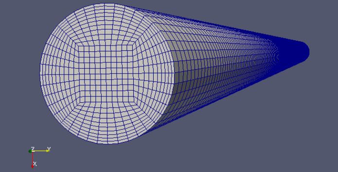
Mesh Manipulation Utilities
The mesh mirroring, creation of a face set using topoSet and creation of patch using createPatch is described below. The original geometry and blockMesh is used from tutorial case incompressible\nonNewtonianIcoFoam\offsetCylinder. The mesh generated by blockMesh utility is shown below. One direct option is to use autoPatch command to split all the face zones based on feature angle. The output is naming of all the patches as auto01, auto02... Once the patches have been generated based on connectivity, renaming of patches can be done in constant/polyMesh/boundary file. Another option is combination of setSet / faceSet and createPatch utility. The third option to use topoSet and creatPatch utilities is explained here.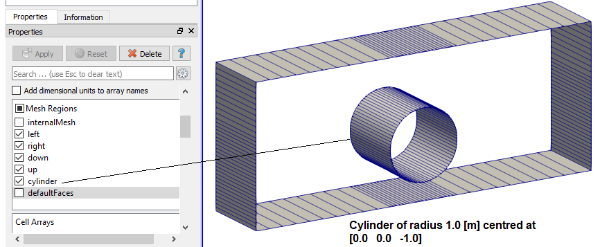
planeType           pointAndNormal;

pointAndNormalDict  {
    basePoint       (0 -1.5 0);
    normalVector    (0  1.0 0);
}
planeTolerance      1e-3;
This resulted in a new mesh with patch name same as original mesh. 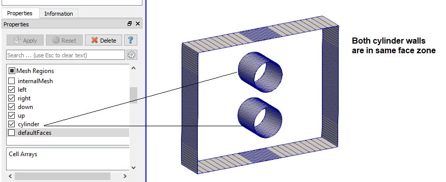
actions
(
// Make a set of all face elements of patch 'cylinder'
{
name cylinderFace; //name of the set
type faceSet; //pointSet/faceSet/cellSet/faceZoneSet/cellZoneSet
action new; //create new, add to existing, delete or subset
source patchToFace; //What is type of 'source' for points/faces/cells
sourceInfo { //method to specify the source
name "cylinder";
}
}
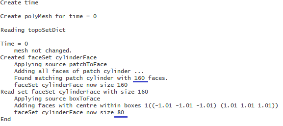
{
name cylinderFace;
type faceSet;
action subset;
source boxToFace;
sourceInfo {
box (-1.01 -1.01 -1.01)(1.01 1.01 1.01);
}
}
);The topoSet utility created a faceSet as shown below.
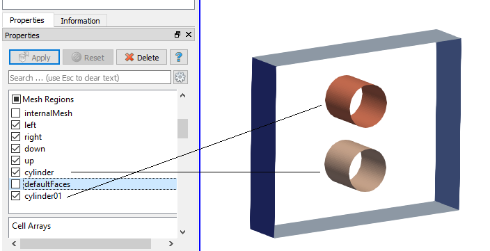
Finally, the createPatch utility was used to create a new patch for upper cylinder.
pointSync false;
patches (   {           // Patches to create.
    name cylinder01;    // Name of new patch
    patchInfo  {        // Type of new patch
      type patch;
    }
    constructFrom set;  //How to construct: either from 'patches' or 'set'
    set cylinderFace;   // name of faceSet created by topoSet
  }
);
Other related utilities are:
- subsetMesh -overwrite c0 -patch newPatch: Here c0 is the cell set defined by topoSetDict. Hence, topoSet or setSet command need to be executed before subsetMesh command. Note that setSet and subsetSet do not require a dictionary.
autoPatch: by default it works on all the boundary (external) faces, no particular faceSet or patch name can be specified.
- With setSet you can define a set of cells (say a rotating domain) interactively - that is directly on command line without need of any dictionary, and then this set of cells can be converted into a zone with setsToZones utility.
Step-by-step guide to use FLUENT Mesh in OpenFOAM
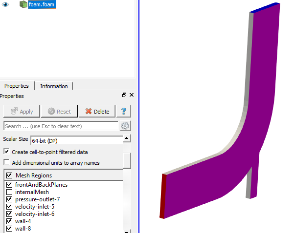
The tutorial file incompressible/icoFoam/elbow contains a sample FLUENT *.msh file. It cannot be viewed in ParaView as it is.Step-01: use utility "FluentMeshToFoam elbow.msh" and convert the mesh data into OpenFOAM format. Create a blank file foam.foam in the main folder which will allow reading the mesh converted into OpenFOAM format. Identify the names of the zones that were defined while generating mesh for FLUENT. e.g. frontAnfBackPlanes, pressure-outlet-7, velocity-inlet-5, velocity-inlet-6, wall-4 and wall-8 in this case.
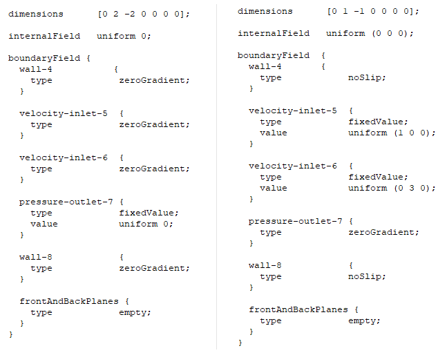
Step-02: Once (FLUENT) zone names are known, define appropriate B.C. on those patches as described below.
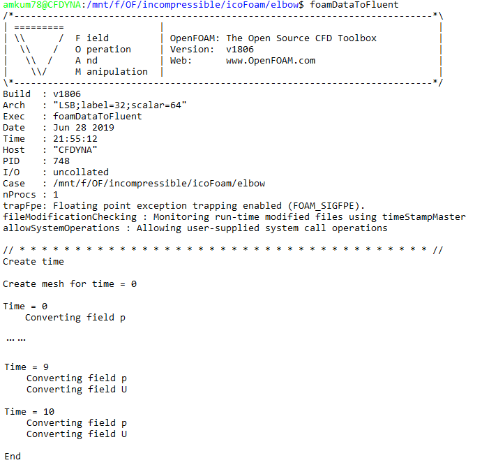
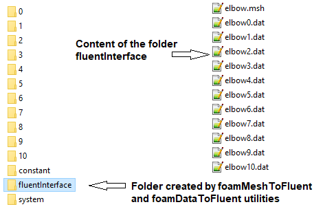
Step-03: Make the simulation run in OpenFOAM. In order to convert the result files back into FLUENT format, use the utilities foamMeshToFluent and foamDataToFluent. Alternatively, the post-processing activities can be carried out directly in ParaView.
Conditionals
Input files support two conditional directives: #if ... #else ... #endif and #ifeq ... #else ... #endif. The #if conditional reads a switch that can be generated by a #calc directive.angle 45.0;
laplacianSchemes {
#if #calc "${angle} < 75"
default Gauss linear corrected;
#else
default Gauss linear limited corrected 0.5;
#endif
}
The #ifeq compares a word or string and executes based on a match.
ddtSchemes {
#ifeq ${FOAM_APPLICATION} simpleFoam
  default         steadyState;
#else
  default         Euler;
#endif
}
References:
- OpenFOAM user manual
- Introductory OpenFOAM Course, from 16th to 20th July, 2018: University of Genoa, DICCA
- Questions and answers on www.cfd-online.com
- OpenFOAM postprocessing and advanced running options: Tommaso Lucchini
- Evoking existing function objects and creating new user-defined function objects for Post- Processing: Sankar Raju N.
- Holzmann CFD
- Introductory OpenFOAM Course - From 16th to 20th July, 2018: University of Genoa, DICCA, Dipartimento di Ingegneria Civile, Chimica e Ambientale
- Computational Fluid Dynamics in OpenFOAM Mesh Generation and Quality: Rebecca Gullberg
- Examples of how to use some utilities and functionObjects (and some Gnuplot, Python, Matplotlib): Hakan Nilsson, CFD with OpenSource Software, 2016
List of Boundary Conditions
The recommended use of variables to define the boundary conditions can be found in folder $FOAM_SRC/ finiteVolume/ fields/ fvPatchField/ derived. E.g. the usage of 'flowRateInletVelocity' boundary type as per header file flowRateInletVelocityFvPatchVectorField.H is as follows.patchName
{
type flowRateInletVelocity;
volumetricFlowRate 0.2;
extrapolateProfile yes;
value uniform (0 0 0);
}
| cylindricalInletVelocity | This boundary condition describes an inlet vector boundary condition in cylindrical co-ordinates given a central axis, central point, rpm, axial and radial velocity |
| fanPressure | This boundary condition can be applied to assign either a pressure inlet or outlet total pressure condition for a fan |
| flowRateInletVelocity | This boundary condition provides a velocity boundary condition, derived from the flux (volumetric or mass-based), whose direction is assumed to be normal to the patch freestream This boundary condition provides a free-stream condition. It is a 'mixed' condition derived from the inletOutlet condition, whereby the mode of operation switches between fixed (free stream) value and zero gradient based on the sign of the flux |
| mappedVelocityFluxFixedValue | This boundary condition maps the velocity and flux from a neighbour patch to this patch |
| outletMappedUniformInlet | This boundary conditon averages the field over the 'outlet' patch specified by name 'outletPatchName' and applies this as the uniform value of the field over this patch |
| pressureDirectedInletOutletVelocity | This velocity inlet/outlet boundary condition is applied to pressure boundaries where the pressure is specified. A zero-gradient condition is applied for outflow (as defined by the flux). For inflow, the velocity is obtained from the flux with the specified inlet direction |
| pressureDirectedInletVelocity | This velocity inlet boundary condition is applied to patches where the pressure is specified. The inflow velocity is obtained from the flux with the specified inlet direction |
| pressureInletOutletVelocity | This velocity inlet/outlet boundary condition is applied to pressure boundaries where the pressure is specified. A zero-gradient condition is applied for outflow (as defined by the flux). For inflow, the velocity is obtained from the patch-face normal component of the internal-cell value |
| pressureInletVelocity | This velocity inlet boundary condition is applied to patches where the pressure is specified. The inflow velocity is obtained from the flux with a direction normal to the patch faces |
| pressureNormalInletOutletVelocity | This velocity inlet/outlet boundary condition is applied to patches where the pressure is specified. A zero-gradient condition is applied for outflow (as defined by the flux); for inflow, the velocity is obtained from the flux with a direction normal to the patch faces |
| pressurePIDControlInletVelocity | This boundary condition tries to generate an inlet velocity that maintains a specified pressure drop between two face zones downstream. The zones should fully span a duct through which all the inlet flow passes |
| rotatingPressureInletOutletVelocity | This velocity inlet/outlet boundary condition is applied to patches in a rotating frame where the pressure is specified. A zero-gradient is applied for outflow (as defined by the flux). For inflow, the velocity is obtained from the flux with a direction normal to the patch faces |
| rotatingTotalPressure | This boundary condition provides a total pressure condition for patches in a rotating frame |
| supersonicFreestream | This boundary condition provides a supersonic free-stream condition |
| surfaceNormalFixedValue | This boundary condition provides a surface-normal vector boundary condition by its magnitude |
| swirlFlowRateInletVelocity | This boundary condition provides a volumetric- OR mass-flow normal vector boundary condition by its magnitude as an integral over its area with a swirl component determined by the angular speed, given in revolutions per minute (RPM) |
| syringePressure | This boundary condition provides a pressure condition, obtained from a zero-D model of the cylinder of a syringe |
| timeVaryingMappedFixedValue | This boundary conditions interpolates the values from a set of supplied points in space and time. Supplied data should be specified in constant/boundaryData/patchname/0 and constant/boundaryData/patchname/points where points contains X, Y, Z coordinates. The default mode of operation (mapMethod with planarInterpolation) is to project the points onto a plane (constructed from the first 3 points), construct a 2D triangulation, find for the face centres the triangle it is in and the weights to the 3 vertices. |
| totalPressure | This boundary condition provides a total pressure condition |
| totalTemperature | This boundary condition provides a total temperature condition |
| turbulentInlet | This boundary condition generates a fluctuating inlet condition by adding a random component to a reference (mean) field |
| turbulentIntensityKineticEnergyInlet | This boundary condition provides a turbulent kinetic energy condition, based on user-supplied turbulence intensity, defined as a fraction of the mean velocity. |
| uniformTotalPressure | This boundary condition provides a time-varying form of the uniform total pressure boundary condition |
| variableHeightFlowRateInletVelocity | This boundary condition provides a velocity boundary condition for multiphase flow based on a user-specified volumetric flow rate |
| variableHeightFlowRate | This boundary condition provides a phase fraction condition based on the local flow conditions, whereby the values are constrained to lay between user-specified upper and lower bounds |
| waveSurfacePressure | This is a pressure boundary condition, whose value is calculated as the hydrostatic pressure based on a given displacement |
| fixedFluxPressure | This boundary condition sets the pressure gradient to the provided value such that the flux on the boundary is that specified by the velocity boundary condition |
| fixedPressureCompressibleDensity | This boundary condition calculates a (liquid) compressible density as a function of pressure and fluid properties |
| freestream | This boundary condition provides a free-stream condition. It is a ’mixed’ condition derived from the i¸nletOutlet condition, whereby the mode of operation switches between fixed (free stream) value and zero gradient based on the sign of the flux |
| freestreamPressure | This boundary condition provides a free-stream condition for pressure. It is a zero-gradient condition that constrains the flux across the patch based on the free-stream velocity |
| mappedFlowRate | Describes a volumetric/mass flow normal vector boundary condition by its magnitude as an integral over its area |
| outletInlet | This boundary condition provides a generic inflow condition, with specified outflow for the case of reverse flow |
| pressureInletOutletParSlipVelocity | This velocity inlet/outlet boundary condition for pressure boundary where the pressure is specified. A zero-gradient is applied for outflow (as defined by the flux). For inflow, the velocity is obtained from the flux with the specified inlet direction |
| pressureInletUniformVelocity | This velocity inlet boundary condition is applied to patches where the pressure is specified. The uniform inflow velocity is obtained by averaging the flux over the patch and then applying it in the direction normal to the patch faces |
| advective / waveTransmissive | This boundary condition provides an advective / wave transmissive outflow condition, based on solving DDt(psi, U) = 0 at the boundary. Note these two B.C. are applicable on patches defined as outlet only. |
Initialization using codeStream: reference "codeStream – Highlights" by WolfDynamics Ltd.
internalField #codeStream { //Use codeStream to set the value of the initial conditions
{
  codeInclude #{
   #include "fvCFD.H"
  #};

  codeOptions #{
   -I$(LIB_SRC)/finiteVolume/lnInclude \
   -I$(LIB_SRC)/meshTools/lnInclude
  #};

  codeLibs #{
   -lmeshTools \
   -lfiniteVolume
  #};

  code #{
   //Access internal mesh information
   const IOdictionary& d = static_cast<const IOdictionary&>(dict);
   const fvMesh& mesh = refCast<const fvMesh>(d.db());
   //Initialize scalar field to zero
   scalarField alpha(mesh.nCells(), 0.);
   scalar he = 0.5;
   scalar ke = 0.5;
   scalar ae = 0.3;
   scalar be = 0.15;
   forAll(alpha, i) {
    //Access cell centers coordinates
    const scalar x = mesh.C()[i][0];
    const scalar y = mesh.C()[i][1];
    const scalar z = mesh.C()[i][2];
	//Assign value to alpha according to conditional structure
    if ( pow(y-ke,2) <= ((1 - pow(x-he,2)/pow(ae,2) )*pow(be,2)) ) {
     alpha[i] = 1.0;
    }
  }
  writeEntry(os, "", alpha);  //Write output to input dictionary
  #};
};
Radiation Modeling
OpenFOAM provides three radiation models: P1 model, fvDOM (finite volume discrete ordinates model) and viewFactor model.If a x L >> 1 then P1 model. If a × L < 1, use of fvDOM is recommended. Since fvDOM also captures the large optical length scales, it is the most accurate model though it is computationally more intensive since it solves the transport equation for each direction. fvDOM can handle non gray surfaces (dependence of radiation on the the solid angle is included). viewFactor method is recommended if non-participating mediums are present (such as spacecraft and solar radiation).
The tutorial heatTransfer\ chtMultiRegionFoam\ externalSolarLoadcase has 3 dictionaries dealing with radiation settings: viewFactorsDict, boundaryRadiationProperties and radiationProperties.
Other tutorial cases dealing with radiation are: heatTransfer\ buoyantSimpleFoam\ hotRadiationRoom, heatTransfer\ buoyantSimpleFoam\ hotRadiationRoomFvDOM and heatTransfer\ chtMultiRegionFoam\ multiRegionHeater.Similarly, a common fvScheme dictionary can be used to cover more than 90% of cases.
The content on CFDyna.com is being constantly refined and improvised with on-the-job experience, testing, and training. Examples might be simplified to improve insight into the physics and basic understanding. Linked pages, articles, references, and examples are constantly reviewed to reduce errors, but we cannot warrant full correctness of all content.
Template by OS Templates