- CFD, Fluid Flow, FEA, Heat/Mass Transfer
Accuracy and correctness
CFD: a complex mix of Physics, Engineering and Art! Results need validation and sanity checks including finding a right mesh through mesh convergence studies!
Validation and Verification of CFD Models
The word "Computational" in the phrase "Computational Fluid Dynamics" is simply an adjective to "Fluid Dynamics". Hence, while dealing with aspects of CFD tool or process, it is vitally important to keep the physical understanding of fluid dynamics uppermost in user's mind as CFD has to do with physical problems. -- Adapted from John D. Anderson, Jr (Computational Fluid Dynamics - The Basics with Applications).
Table of Contents:
Velocity Profile in Natural Convection [+] Heat Transfers from Extended Surfaces (Fins) {*} Optimum Spacing of Heat Sink (*) Example of Engineering Assumptions (+) Estimation of Error (*) Sources of Errors {+} Types of errors {=} Benchmarking and CalibrationEverybody believe an experiment, except the one who did it.
Nobody believes a simulation result, except the one who did it.
We have all come across the phrase "garbage in, garbage out" which has originated from software development (attributed to be coined by George Fuechsel, an IBM programmer and instructor). However, this is equally valid for any 'computer' program where the validity of input decides the correctness of the output. In case of CFD simulations, the term 'validity' refers to the "appropriateness and accuracy" of the input data for numerical simulations. Validation of CFD models is a necessity. These numerical tools are used for different applications and no internal checks are implemented inside the program for the correctness of CFD results. Hence, anybody and everybody who are using CFD simulation tools must make "validation of CFD results" an integral part of their simulation process and activities.

Any numerical simulation process is not just "Meshing, setting Boundary Conditions, Running Solver and Making Colourful Contour / Vector Plots". The results ultimately needs to be converted into a set of inputs for a robust design of the components or sub-systems of a system. The results of any numerical simulations need to be critically and thoroughly analyzed for errors, omissions and inaccuracies.
A sound knowledge of "underlying fluid mechanics principles and operating conditions of the problem set-up" are more important than just knowing how to use the software. Some of the topics which will help "CFD practitioners" make correct and robust design decisions based on CFD results are:
- Basic of fluid mechanics such as Bernoulli's equation and actual physics behind this principle
- Fluid mass, momentum and energy conservation with underlying mathematics
- Shear stress formulation on fluid flow, empirical correlations, testing methods and correlations with experimental data
- Flow behaviour such as developing flow, developed flow, no-slip condition, separation and re-attachment
- Complete theoretical and experimental behaviour of following flow conditions:
- Flow inside a circular duct
- Flow over a circular cylinder
- Flow over a flat plate
- Flow between two parallel plates
- Natural convection in an enclosed cavity
Though the industrial flow configurations are far from being closer to these simple geometries, the fundamental ideas contained in them are indispensable to a good understanding of modern computational methods. The methods and results arrived at are important not only for these simple flows but also for the extension of our fundamental knowledge of turbulent flows in general. Methods for dealing with turbulent flows for any industrial applications could be devised only on the basis of the detailed experimental results obtained for them.
For example, according to measurements performed by H. Kirsten, the entrance length of a turbulent flow in a pipe is about 50 to 100 diameters. This knowledge is very important in deciding the inlet boundary condition for any industrial internal flow configuration.
CFD: Computational or 'Colourful' Fluid Dynamics?
CFD is a great tool when used with appropriate procedure and guidelines because of its inherent nature of multi-disciplinary science leading to technically unlimited potential and applications. Yet, "CFD is not a panacea of all the Flow and Heat Transfer problems without experience-base insight". Any result must be looked at by an experienced engineer in that field and must go through an "order-of-magnitude-check" before accepting the results.
- CFD simulations are capable of predicting good qualitative results (trends). It will not make decisions for design engineers but certainly help them take more informed judgment. When no information is available about flow structure in a system, CFD is certainly an economical start into detail analysis of the performance of the system.
- Even inaccurate CFD results, so long it is ensured mathematically physical, possesses many features which make it very useful:
- The sheer capability of detailed visualization is rich in information.
- CFD results give an insight which is not possible by experiments and other theoretical means.
- Trends are usually reliable and leads to right direction in terms of design evaluations.
- In many cases, quantitative information is predicted with sufficient accuracy to justify engineering design changes on commercial plant. CFD can even predict more useful information than testing because the measurement point (typically based on user experience) may not be at appropriate location.
- Historical knowledge obtained from plant operation is a great validation tool for such numerical (or virtual) simulation results.
- Notwithstanding the limitations mentioned above, CFD models drastically reduce implementation of "Design Modifications and Scale-up of a System"
- CFD can be also used early in the design stage for performance evaluation, for optimization and enhancement during the development stage and for diagnostics in the later stage of the produce development cycle.
All methods for the calculation of turbulent boundary layers are approximate ones and are based on the integral forms of the momentum and energy equations. Since, however, no general expressions for shear and dissipation in turbulent flow can be deduced by purely theoretical considerations, it is necessary to make additional suitable assumptions. These can only be obtained from the results of systematic measurements and, consequently, the calculation of turbulent boundary layers is semi-empirical.
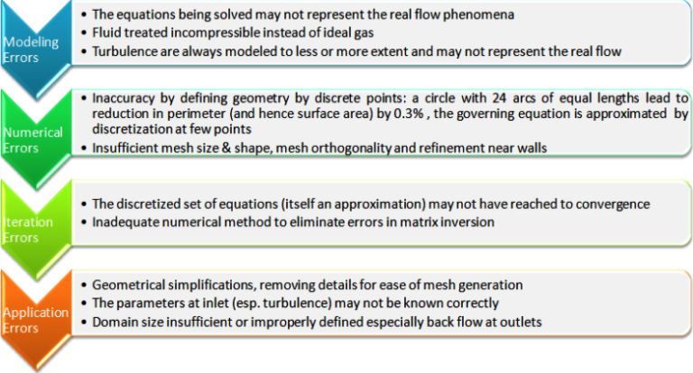
While the usage of CFD simulations in industry is on rise at rapid pace, the credibility of results of any such calculation is still an area of concern. Most organizations using such codes, over time have evolved their own best practice guidelines to minimize the chances of "critical errors". There are many such guidelines issued by ERCOFTAC and AIAA. Following diagram summarizes classifications used to designate the types of error which needs to be addressed when CFD simulations are used to make decisions on performance of a product.
Example of Engineering Assumptions
Sources of Errors
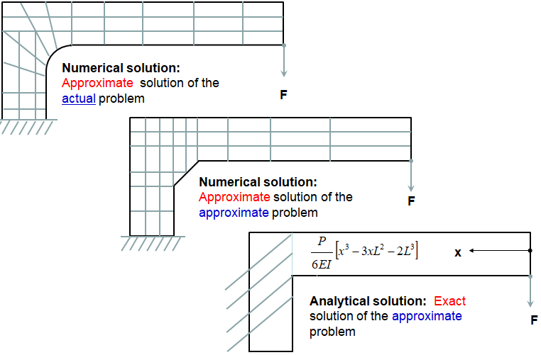
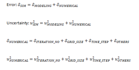
When a numerical model is created to get a solution, a 'model' is created and not a exact copy or a 'replica'! That is, there is an inevitable deviation "between the real flow and the model" and "between numerical solution of governing PDEs and the exact solution" of the model. As per AIAA:Error: A recognisable deficiency that is not due to lack of knowledge. For example, common known errors are the round-off errors in a computers and the convergence error in an iterative numerical scheme. CFD analyst should be capable of estimating the likely magnitude of the error. It may also arise due to mistakes in input (such as material property variation with temperature).
Uncertainty: A potential deficiency that is due to lack of knowledge. Uncertainties arise because of incomplete knowledge of a physical characteristic, such as the turbulence structure at inlet to a flow domain or because there is uncertainty in the validity of a particular flow model being used. Uncertainty cannot be removed as it is rooted in lack of knowledge (wither physics of the flow or the behaviour of numerical codes). Statistically, the uncertainty of the observable X is a measure of the spread of results around the mean X, also designated as standard deviation.
Verification: It is the procedure intended to ensure that the program solves the equations correctly. As per AIAA, G-077-1998: the process of determining if a simulation accurately represents the conceptual model. A verified simulation does not make any claim relating to the representation of the real world by the simulation. In other words, as per Roache: "it solves the equations right".
Validation: This procedure is intended to test the extent to which the model accurately represents reality. As per AIAA, G-077-1998: it is the process of determining how accurately a simulation represents the real world. In other words, as per Roache: "it solves the right equations".
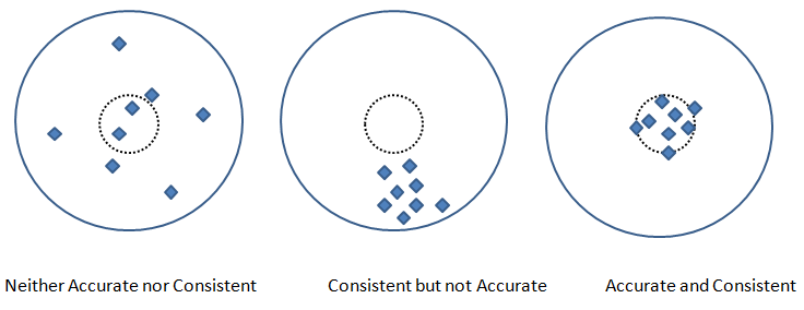
Accuracy: This is the measure of the similarity of a simulation to the physical flow it is expected to represent. It represents how a predicted value is closer to the measured and/or theoretically exact value.
Consistency: This refers to the 'repeatability' of a process, be it testing or simulation. In measurement or manufacturing process, there are methods for "Gauge R&anp;R" which stands for repeatability (same output by same operator under identical operating conditions) and reproduceability (same output by different operator) of a method.
Calibration: This procedure to assess the ability of a CFD code to predict global quantities of interest for specific geometries of engineering design interest.
Types of errors
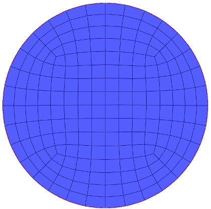
- Numerical Errors / Discretization Error: It is difference between "exact solution of the conservation equations" and the "exact solution of the algebraic set of discretized equations". The two most effective strategies to reduce this tyoe of errors are (i) increasing the order-accuracy of discrete approximations (e.g. using the high resolution such as central-difference scheme rather than the upwind difference advection scheme) and/or (ii) by reducing the element size in regions of rapid solution variation.
Due to discretization of curved or circular edges (tessellated boundaries), the area is reduced as compared to the curved boundaries. If a velocity boundary condition is being used, it needs to be scaled up in the ratio of reduction in area. Remedy: Grid Convergence Study.
- Modeling Errors: Defined as the difference between the actual flow and the exact solution of the mathematical model. This error arises due to assumptions made in deriving the transport equation, simplification of the geometry of the solution domain. Remedy: These errors are not known a priori, they can only be evaluated by comparing solutions in which the discretization and convergence errors are negligible with accurate experimental data.
- Iteration Errors: It is difference between 'iterative' and 'exact solution' of discretized algebraic equation. Remedy: Exploiting the solver control parameters to get a convergence for different levels of residual such as 1.0E-03, 1.0E-04, 1.0E-05.
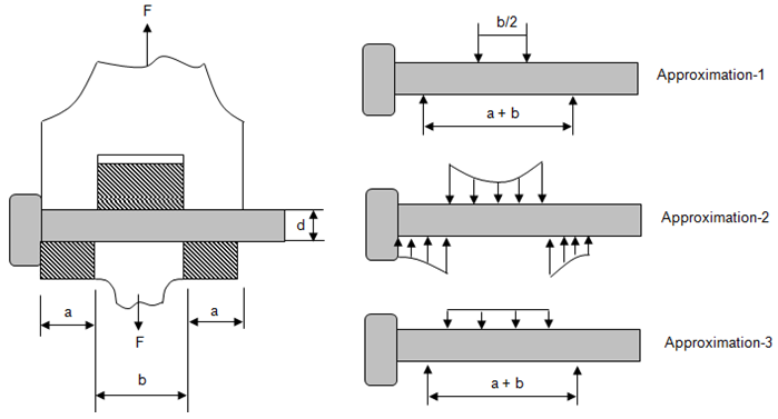
- User Error and Application Uncertainties: Wrong selection of turbulence model, insufficient Information about BC setting, poor quality grid generation and boundary layer resolution. Remedy: These can be minimized through experience, Best Practice Guidelines (BPG) and optimization of resources. For example, the mesh of a circular cross-section seems to capture the circumference well. However, a closer look reveals that cross-section area of discretized face is lower than that of a circle.
Thus, inlet velocity calculated based on known mass flow rate and area of a circle needs to be adjusted to account for reduction in actual area of the meshed surface.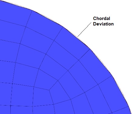
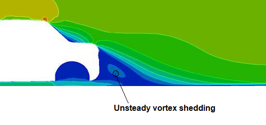
Examples of errors in an External Aerodynamics Simulation: External flow over a car is similar to flow over a bluff-body and hence formation of wake region is an inevitable part of the simulation. Such wake regions have flow field which are inherently unsteady in nature. Hence, any steady state flow simulation may not capture the interaction between the wake region with rest of the flow field. However, steady state simulation method has its own advantages such as low simulation run-time ideally suited for optimization studies to reduce drag. The accuracy in absolute values and trends are reasonably good and consistent.
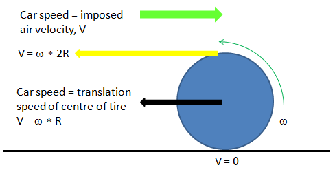
Similarly, not modelig the rotation of the tires and simplification of tire surfaces by removing the grooves can be significant source of error with respect to the actual driving conditions. However, in wind-tunnel tests, the car body is stationary and tyre may not be rotating (though it can be made rotating) - the CFD simulation result will be closer to the test result.
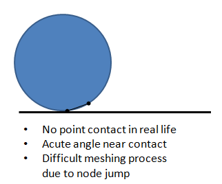
Cases like this when there is rotational contact between two surfaces, the contact area is not correctly known or sometimes it cannot be capture correctly due to accute angle between the circular disk and flat plate.
In actual driving conditions, car is moving through stationary air and the boundary layer may not form at the road surface. When air is blown over a stationary car in wind tunnel testing and CFD simulations, boundary layer forms on the surface representing the ground/road. The remedy is to apply moving wall to the floor having velocity same as car speed.
External aerodynamics simulations are sensitive to the quality of the surface geometry representation. Care must be taken when using the surface wrapper such that junctions/intersections result in smooth and well-defined edges. The geometry simplifications such as removal of small protrusions, deletion of thin wires, smoothen of surface undulation... should be carried out judiciously. Normally such clean-up is a compromise in ability to generate good quality mesh and loss in accuracy due to simplifications. In other words, keeping some of the geometrical features may result in distorted and skewed cells which anyways reduce the accuracy of simulation results.
Recommended monitor points to check for convergence for external aerodynamic simulation over a car body:
- Force or average shear stress on BIW surfaces: this monitor reaches a steady value at convergence.
- Pressure probes in tire and vehicle wake: a variation within ±10% to mean convergence value is accurate enough for drag and lift prediction. Note that this assumes that the mean line is flat over last 100-500 iterations.
Steps to check and increase accuracy of CFD results
- Step-01: use of monitor points - use monitor points relevant to the simulation physics to check if simulation is proceeding "as expected". The term "as expected" has been to emphasize the fact that one should always have some idea what he is expecting from a CFD simulation!
- Step-02: compatibility of wall function and area-averaged y+ value - each type of wall function developed has certain requirement on boundary layer resolutions. Ensure that the area-averaged values on all the walls fall in that range - area-averaged because it is not always possible to maintain the y+ in a certain range for every location of the walls.
- Step-03: sensitivity to mesh size - you have chosen a particular mesh size on walls and in the fluid region based on some reference or past experience or even due to constraints on available hardware (machine RAM size and CPU speed). It is advisable to first check the effect of element sizes on a mesh coarser by two times the baseline mesh.
MESH CONVERGENCE STUDY: The formal method of establishing mesh convergence requires a curve of a critical result parameter (typically some kind of coefficient such as skin friction coefficient) in a specific location, to be plotted against some measure of mesh density. At least 3 simulation runs are required to plot a curve which can then be used to indicate how convergence is achieved or how far away the most refined mesh is from full convergence. However, if two runs of different mesh density give the same result, (mesh) convergence must already have been achieved and no mesh convergence curve is necessary. Yet, one must be aware that 2 sets of results will only indicate sensitivity and not the mesh convergence.
Another key parameter of a mesh convergence study is the refinement ratio (> 1.0). It is defined as the ratio between two consecutive refinement levels. The use of uniform parameter refinement ratio is recommended for a given parameter. Different refinement ratio for different parameters can also be used based on past experience of the importance of change in value on simulation results. For most of industrial applications with moderate level of accuracy requirements, a refinement ratio of 2.0 often is too high - e.g. it may either lead to a very fine or a very coarse mesh for one of the minimum 3 cases required for convergence study. A refinement ratio of sqrt(2) or 1.5 is a good compromise to distinguish convergence study with iterative errors.
Define target variables (usually scalars like Force, Drag Coefficient, Heat Flux, HTC, MAX Temperature...). Check the variation in target variable (e.g. mass flow rate at any plane) for various refinements of mesh, keep ITERATION ERROR limit constant say 1.0E-4
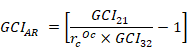
Let's take an example of pump where target variable is head developed by the pump. 3 different meshes are generated with refinement ratio rc = 1.5. Let H1, H2 and H3 are heads calculated in increasing or decreasing order of refinement. The order of convergence is expressed as: Once the order of convergence is obtained, the average head at zero grid spacing, H(δx = 0) can be determined using a Richardson extrapolation of the two finest mesh. The Grid Convergence Index (GCI) proposed by by Roache (1994) using a safety factor Fs of 1.25 should be calculated for mesh pairs [2, 1], [3, 1] and [3, 2].
How close the solution is within the asymptotic range can be calculated using following expression. The value closer to 1 indicates closeness to the asymptotic range.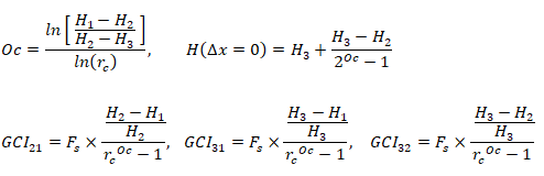
- Step-04: Effect of inlet boundary condition say effect of turbulence values at inlet - most of the time the turbulence value specified at inlet face is a guess, say turbulence viscosity ratio = 5 and turbulent intensity = 10. Do we know where these values have come from? Check if the results are affected with these values are doubled or halved. Ideal situation would be to have the turbulence level based on measurements but it is not always the case.
In addition to the turbulence parameter, the inlet velocity profile itself is very important to study the accuracy of CFD result for a particular application. One should check the effect of velocity profile as per power-law such as u = UMEAN*(y/d)1/n, where n = 6, 7, 8, … depending upon Re value. These sensitivity studies are particularly important in cases where separation and reattachment are likely to occur. For Example, in case of a flow over Backward Facing Step, there is decreases in location of reattachment length as the turbulence intensity increases and is sensitive to TI value specified at inlet.
- Step-05: effect of temperature dependent material properties - this is important especially when the temperature gradients are 'large' or the change in pressure is such that it can lead to 'significant' change in density of gas. The value of 'large' and 'significant' used here changes across the applications, a value of 10% is considered to be 'significant'.
- Step-06: extraction of quantitative values and interpretation of results - sometimes the way area-averaged or surface integrals are calculated, they need to be interpreted appropriately. For example, even in case of a constant area duct with water as incompressible constant property fluid, the change in static pressure between inlet and outlet will not be same as change in total pressure.
- Why? As the area is same and fluid is incompressible, the expected changed in dynamic head (velocity pressure) is zero!
- The explanation lies in the way area-averaged or mass-averaged dynamic head is calculated at outlet where flow is not uniform whereas the specified velocity field at inlet is uniform.
Estimation of Error
Adapted from "VERIFICATION AND VALIDATION OF CFD SIMULATIONS" by Fred Stern, Robert V. Wilson, Hugh W. Coleman, and Eric G. Paterson: Error δ is the difference between a [simulation value] or an [experimental value] and the [true value]. The true values of any simulation and/or experimental quantities are rarely known. Thus, errors must be estimated. An uncertainty U is an estimate of an error such that the interval ±U contains the true value of δ, say 95% of times. An uncertainty interval thus indicates the range of likely magnitudes of δ but no information about its sign.Sources of errors and uncertainties in results from simulations can be divided into two distinct sources: modeling and numerical. Modeling errors and uncertainties are due to assumptions and approximations in the mathematical representation of the physical problem (such as geometry, mathematical equation, coordinate transformation, boundary conditions, turbulence models, etc.) and incorporation of previous data (such as fluid properties) into the model. Numerical errors and uncertainties are due to numerical solution of the mathematical equations (such as discretization, artificial dissipation, incomplete iterative and grid convergence, lack of conservation of mass, momentum, and energy, internal and external boundary non-continuity, computer round-off...).
Best Practice Guidelines (BPG): A Quality Assurance Approach
There is no unique method or approach to CFD simulations universally applicable to all industries and all types of flow and heat transfer problems. Hence, specific to applications and industry, best practice guidelines have been evolved by the users as well as the software vendors. These guidelines are also called "quality assurance method" because they remove user-dependencies and make the simulation deterministic to large extent.Buoyancy-driven Flows
Such flows are difficult to converge and special attention is needed to set-up the solver. Buoyancy driven flow can be of two types: (a) Open boundaries and (b) Closed domain. While modelling natural convection inside a closed domain, the solution depends on the mass inside the domain. Since the mass in the domain will be known only if the density is known, one must model the flow in one of the following ways:- When change in temperature of fluid is high causing variation in density ≥ 10%: Perform a transient calculation since the initial density will be computed from the initial pressure and temperature, so the initial mass is known. As the solution progresses over time, this mass is conserved.
- When change in temperature of fluid is small such that variation in density < 10%: Perform a steady state simulation using the Boussinesq model where user needs to specify a constant density, so the mass of the system is properly specified. As the solution progresses over time, this mass is conserved.
Sample Checklist
- Has the outlet boundary location selected sufficiently far away from wake-regions and domain of interest?
- Has a suitable monitor such as "wall shear stress" on area of interest been used to assure proper convergence?
- Has the turbulent intensity at inlet(s) been set as per expected operating conditions?
- Has the selection of 'steady state' or 'transient' simulation method been made keeping in mind wake region and vortex-shedding frequency?
- Has the reverse flow, if any, been maintained less than 5% of the outlet area? Has appropriate pressure or temperature of reverse flow been set?
- Does the wall y+ conform to the recommended range for the wall function used?
- Has discretization schemes been used second order for flow and temperature fields? For some applications, has FLUENT's recommended QUICK scheme used for pressure?
- Has the "Radial Pressure Equilibrium" at rotating wall been turned on if it intersects "pressure outlets"? Applicable to ANSYS FLUENT only.
- Has reference density for fluid defined correctly for buoyant flows? Does the reference location fall inside computational domain?
- Has the option of steady-state calculation using the Boussinesq model been chosen keeping in mind small temperature difference in the domain: such that variation in density is within ±10% of maximum density expected in the system?
In ANSYS FLUENT and as a matter of fact all CFD programs, heat transfer coefficient (h) is a derived quantity using wall temperature, adjacent fluid temperature and heat flux. Note the term "adjacent fluid temperature". This approach makes the HTC value reported by post-processing programs only indicative. In reality: one should estimate heat flux value (q") and area-weighted average temperature (TW_MEAN) from post-processing utility. Then use the equation: q" = h·(TW_MEAN - TREF) to estimate h. Here selection of TREF should be made inline with empirical correlations reported in text-books.
Database of major errors
| S. No. | Description of error | Cause or reason of occurrence | Impact of error |
| 01 | Incorrect use of material properties especially thermal conductivity | Skill and ignorance | Re-run with schedule and budget over-run |
| 02 | Incorrect boundary location and type for buoyancy-driven flow resulting in primary flow along the direction of gravity | Lack of understanding about physics of natural convection | Unwanted change in design due to incorrect result |
| 03 | Missing contact between heat generating block and heat spreader leading to high temperature predictions | No self-check during pre-processing or post-processing | Multiple reviews and delays in design freeze |
| 04 | Demanding inputs from customer not required for (steady state) simulations | Competency and knowledge | Customer's displeasure and impact on future business |
| 05 | Ignoring conduction heat transfer through high conductivity but thin wires | Unintentional overlook and very conservative estimation | Many design iterations leading missed milestones |
| 06 | Terminating the run based on iterations, before monitor points stabilized | Transfer of ownership from one person to another | Delay and question mark on team's capabilities |
| 07 | Making multiphase flow simulations based on ad-hoc assumptions and common sense* | Lack of knowledge about solver capabilities | Delay and unpaid efforts |
| 08 | Wrong selection of hub and shroud walls for a simulation of turbo-machine | Technical oversight | Rework and extra unpaid effort |
| 09 | Wrong interpretation of results where a transient phenomena was converted into steady state | Not able to convey the physics to design engineer | Extra iterations though paid by customer |
| 10 | Not modeling thermal radiation for a passive cooling phenomena | Competency | Rework (more machine time) |
Benchmarking and Calibration
The CFD simulations have not reached to a stage where it can completely eliminate the test. A calibration of CFD model is needed for every design evaluation case which can be used on subsequent design iterations with high probability of success in physical tests. Benchmarking and calibration are many a times used interchangeably though they are not the same in strict sense.Method of Calibration
- Step-1: Gather the information about test set-up, test geometry and measurement records [location of measurement, type of measurement]
- Step-2: Check the possibility of additional measurements as only few measurement points may not be sufficient to calibrate a CFD simulation model
- Step-3: Carry out CFD simulations with different mesh resolutions at walls, turbulence models and discretization schemes till the computed value match the test values within specified limits.
What equations are used by programs?
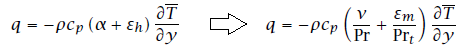
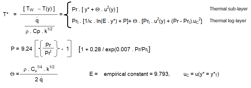
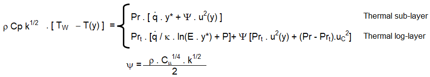
An understanding of how the program evaluates quantitative information such as wall shear stress, heat flux, heat transfer coefficient...is also important to identify the source of error. The wall shear stress is strongly dependent on the turbulence modeling and wall functions used. The information related to tubulence modeling can be access on the this page.Heat flux and surface heat transfer coefficient is one of the critical output from a thermal simulation. Understanding of the temperature field near the wall and how its gradient is used to calculate the heat transfer rate is important to identify source of errors. Heat transfer at walls is a combination of "heat diffusion due to conduction" and "heat diffusion due to mixing or convection". This is expressed as described below. Here, T is 'local' time-averaged value. α is thermal diffusivity defined as k/ρCp, εh is eddy diffusivity of heat - analogous to eddy diffusivity of momentum.
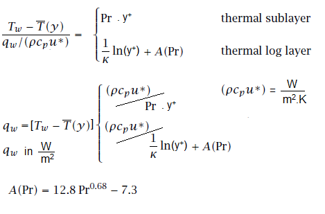
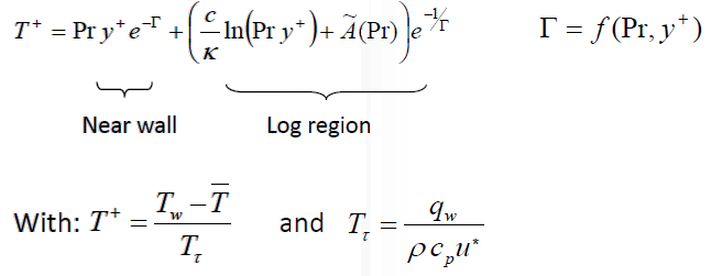
Step-1: Molecular Prandtl number is calculated based on specified fluid properties: Pr = μ / Cp / k where k is thermal conductivity (not turbulent kinetic energy though k used in law of wall for temperature above is TKE)
↓
Step-2: For the calculated molecular Prandtl number, thermal sub-layer thickness is estimated which is nothing but the intersection of the linear and logarithmic profiles
↓
Step-3: Depending upon (momentum) boundary layer height, y* is calculated at the centroid of the near wall cell. As mentioned above, in FLUENT, the laws-of-the-wall for mean velocity and temperature are based on the wall unit y* rather than y+.
↓
Step-4: Once y* is calculated, velocity at the centroid of the near wall cell is calculated as per law-of-wall for velocity. Thus, Pr, y* and u(yP) are calculated and stored now. Temperature at near wall cell is, T(yP) still not known.
↓
Step-5: T(yP) is known by solution of of energy equations in the interior domain. For specified wall temperature boundary condition, heat flux is calculated from the linear equation arising from the law-of-the-wall.
Sanity check: HTC
Following calculation is based on Gnielinski correlation which is valid for transition and fully-turbulent flows. The Nusselt number of laminar flows in pipe is 3.657 for constant wall temperature and 4.364 for constant wall flux conditions. 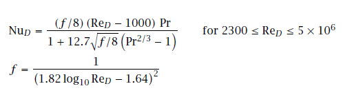
| Select the type of geometry: | |
| Select the working fluid: | |
| Select mode of specifying velocity scale: | |
| Specify velocity scale in [m/s] or [m3/s] or [kg/s]: | |
| Specify cross-section area in [m2] - ignored if velocity is specified: | |
| Select wall condition: 1=constant temperature, 2=constant heat flux: | |
| Select wall temperature: | |
| Specify length scale of flow: hyd. dia. (Ducts and bluff bodies) or length of the (Flat) plate [m]: | |
| Specify working temperature of the fluid in [°C]: | |
| Specify 'absolute' working pressure (required in case of air only) in [bar]: | |
| Heat transfer type: 1=Force convection, 2=Natural convection: | |
Nusselt number of Nu = 1 for an enclosure corresponds to pure conduction heat transfer through the enclosure. The air in the enclosure in this case remains still, and no natural convection currents occur in the enclosure. Nusselt number > 1 indicates that heat transfer through the enclosure is that much times more than that by pure conduction. The increase in heat transfer is due to the natural convection currents that develop in the enclosure.

Velocity Profile in Natural Convection: referenced from "A Textbook of Heat Transfer" by S. P. Sukhatme

| ν [m2/s] | Pr | g [m2/s] | TW [°C] | TAMB [°C] | TMEAN [°C] | β [1/K] | C0 | C1 | C2 |
| 1.75E-05 | 0.7241 | 9.806 | 70 | 20 | 45 | 0.00314 | 6.984E-05 | 5.255 | 5.027E+07 |
δ = 0.0624 * x0.25 and Vx1 = 0.4952 * x0.50 where y must be ≤ δ. The velocity is maximum at y = δ / 3.
| x [mm] | 50 | 50 | 50 | 100 | 100 | 100 | 200 | 200 | 200 |
| δ [m] | 0.02951 | 0.02951 | 0.02951 | 0.03509 | 0.03509 | 0.03509 | 0.04173 | 0.04173 | 0.04173 |
| δ [mm] | 29.5 | 29.5 | 29.5 | 35.1 | 35.1 | 35.1 | 41.7 | 41.7 | 41.7 |
| y [m] | 0.010 | 0.020 | 0.0295 | 0.015 | 0.030 | 0.0351 | 0.020 | 0.030 | 0.0417 |
| Vx [m/s] | 1.640E-02 | 7.791E-03 | 6.479E-09 | 2.194E-02 | 2.817E-03 | 1.247E-08 | 2.878E-02 | 1.258E-02 | 1.098E-07 |
| Vx [mm/s] | 16.4 | 7.8 | 0.0 | 21.9 | 2.8 | 0.0 | 28.8 | 12.6 | 0.0 |
Sample calculation to get order of magnitude for heat transfer rate in natural convection cases with air as cooling medium: example from Heat and Mass Transfer Fundamentals and Applications by Cengel and Ghajar.
Horizontal Cylinder: 8 [cm] diameter with wall temperature at 70 [°C] and ambient temperature at 20 [°C]

Vertical Plate: Square plate of side length 60 [cm] held at 90 [°C] in air at 30 [°C]

Horizontal Plate heated from Top and Bottom: Square plate of side length 60 [cm] held at 90 [°C] in air at 30 [°C]

Equivalence of Radiative Heat Transfer Rate at Low Temperature and Small Temperature Differences
Convective heat transfer rate: qCNV'' = h x [T - TREF].Radiative heat flux rate: qRAD'' = ε x σ x [TW14 - TW24] = ε x σ x [TW1 - TW2] x [TW1 + TW2] x [TW12 + TW22]
Comparing the two equations: hRAD ≡ ε x σ x [TW1 + TW2] x [TW12 + TW22]
For ε = 1.0, TW1 = 100 [°C] and TW2 = 40 [°C], hRAD = 9.23 [W/m2.K]For ε = 1.0, TW1 = 80 [°C] and TW2 = 40 [°C], hRAD = 8.41 [W/m2.K]
For ε = 1.0, TW1 = 60 [°C] and TW2 = 50 [°C], hRAD = 8.01 [W/m2.K]
As you can see, the convective heat transfer coefficient in natural convection with air ranges between 5 to 15 [W/m2.K]. Hence, the contribution of radiation in natural convection cases (such as electronic cooling) is approximately equal to the convective heat transfer rate. In other words, convection and radiation contribute almost equal in natural convection heat transfer cases dealing with low temperature differences.
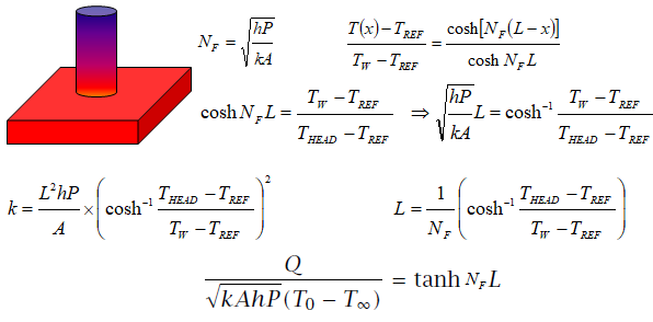
Heat Transfers from Extended Surfaces (Fins)
This section provides a way to calculate heat transfer rate and estimate typical range of values for designs. Two design criteria used to define performance of fins are "fin efficiency" and "fin effectiveness". Fin efficiency is ratio of "actual heat transferred through fins" to the "heat that would be transferred if the entire fin were as base temperature". 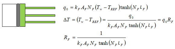
| BF | Thickness of fins | [mm] | 1 | 2 | 2 | 2 | 5 | 5 |
| LF | Height of fins | [mm] | 20 | 20 | 10 | 20 | 20 | 10 |
| WF | Width of Al-fins | [mm] | 250 | 250 | 250 | 250 | 100 | 100 |
| AF | Cross-section of fins | [mm2] | 250 | 500 | 500 | 500 | 500 | 500 |
| PF | Perimeter of fins | [mm] | 502 | 504 | 504 | 504 | 210 | 210 |
| kF | Thermal conductivity of fin | [W/m-K] | 100 | 100 | 100 | 100 | 100 | 100 |
| h | Convective Heat Transfer Coefficient | [W/m2-K] | 10 | 10 | 10 | 10 | 10 | 10 |
| NF | Fin parameter | [m-1] | 14.17 | 10.04 | 10.04 | 10.04 | 6.48 | 6.48 |
| RF | Thermal resistance of each fin | [K/W] | 10.23 | 10.05 | 19.91 | 10.05 | 23.94 | 47.69 |
| iF | Number of fins | [nos] | 10 | 10 | 10 | 10 | 10 | 10 |
| RF | Thermal resistance of all fins | [K/W] | 1.02 | 1.01 | 1.99 | 1.01 | 2.39 | 4.77 |
| ΔT | Temperature potential | [K] | 60 | 60 | 60 | 60 | 60 | 60 |
| Q | Heat transfer rate | [W] | 58.7 | 59.7 | 30.1 | 59.7 | 25.1 | 12.6 |
| A | Heat transfer surface area | [cm2] | 10 | 10 | 5 | 10 | 4 | 2 |
| ΔT/[A.Q] | Heat transfer rate | [K/W/m2] | 0.102 | 0.101 | 0.398 | 0.101 | 0.599 | 2.384 |
| Select the type of Fin: | |
| Thermal conductivity of fin in [W/m-K]: | |
| Specify length or height of fin [mm]: | |
| Diameter (pin-type) or thickness (plate-type) of fin [mm]: | |
| Width of plate-type fin [mm]: | |
| Convective HTC on fin surface [W/m2.K]: | |
| Reference temperature [°C]: | |
| Base temperature [°C]: | |
| Base thickness [mm]: | |
| Tip convection [W/m2.K]: | |
The heat transfer rate of pin-type fin for natural convection in air is tabulated below. Note the impact of L/D ratio on heat transfer rate.
| L | [mm] | 100.0 | 100.0 | 100.0 | 100.0 | 100.0 | 100.0 | 100.0 |
| D | [mm] | 5.0 | 10.0 | 20.0 | 25.0 | 50.0 | 100.0 | 200.0 |
| h | [W/m2-K] | 10.0 | 10.0 | 10.0 | 10.0 | 10.0 | 10.0 | 10.0 |
| ΔT | [K] | 60.0 | 60.0 | 60.0 | 60.0 | 60.0 | 60.0 | 60.0 |
| NF | [m-1] | 8.9 | 6.3 | 4.5 | 4.0 | 2.8 | 2.0 | 1.40 |
| A | [cm2] | 15.7 | 31.4 | 62.8 | 78.5 | 157.1 | 314.2 | 628.3 |
| Q | [W] | 0.7520 | 1.6680 | 3.5370 | 4.4760 | 9.18 | 18.60 | 37.45 |
| ΔT/[A.Q] | [K/W/cm2] | 5.079 | 1.145 | 0.270 | 0.1707 | 0.0416 | 0.0103 | 0.0025 |
The values for forced convection in air is tabulated below. 'A' is the heat transfer area of the fin and not the cross-section area. The parameter ΔT/[Q.A] can be used in fin selection for given heat dissipation and surface area (available space). For example, for a heat dissipation of 10 [W] using a fin of diameter 20 [mm] and height 100 [mm], the expected increase in temperature of the base of fin is 10 [W] x 62.8 [cm2] x 0.1431 = 89.9 [K].
| L | [mm] | 100.0 | 100.0 | 100.0 | 100.0 | 100.0 | 100.0 | 100.0 |
| D | [mm] | 5.0 | 10.0 | 20.0 | 25.0 | 50.0 | 100.0 | 200.0 |
| h | [W/m2-K] | 20.0 | 20.0 | 20.0 | 20.0 | 20.0 | 20.0 | 20.0 |
| ΔT | [K] | 60.0 | 60.0 | 60.0 | 60.0 | 60.0 | 60.0 | 60.0 |
| NF | [m] | 8.9 | 6.3 | 4.5 | 4.0 | 2.8 | 2.0 | 1.40 |
| A | [cm2] | 15.7 | 31.4 | 62.8 | 78.5 | 157.1 | 314.2 | 628.3 |
| Q | [W] | 1.270 | 3.008 | 6.673 | 8.533 | 17.905 | 36.725 | 74.409 |
| ΔT/[A.Q] | [K/W/cm2] | 3.0070 | 0.6350 | 0.1431 | 0.0895 | 0.0213 | 0.0052 | 0.0013 |
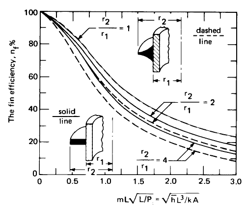
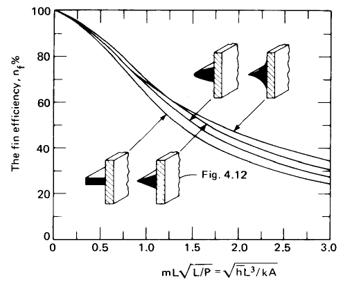
The chart below provides a comparison between two designs of circular fins. Here, L ≡ r2 - r1 and 'A' is based on section shaded in dark colour. Reference: A Textbook of Heat Transfer by Lienhard and Lienhard.
Optimum Spacing of Heat Sink
The optimum fin spacing for a vertical heat sink is given by Rohsenow and Bar‐Cohen as described below. L is the characteristic length in Ra number. All the fluid property are determined at the film temperature (average of wall temperature and free-stream temperature) which means that final temperature calculation is an iterative process.

Filling and Emptying Process of Gases
For theoretical formula: "Fundamentals of Engineering Thermodynamics" By E. Rathakrishnan, pages 68-69. For numerical investigation: Kawano Y et al. "Thermal analysis of high-pressure hydrogen during the discharging process", International Journal of Hydrogen Energy - images from paper shown below.
The content on CFDyna.com is being constantly refined and improvised with on-the-job experience, testing, and training. Examples might be simplified to improve insight into the physics and basic understanding. Linked pages, articles, references, and examples are constantly reviewed to reduce errors, but we cannot warrant full correctness of all content.
Template by OS Templates