- CFD, Fluid Flow, FEA, Heat/Mass Transfer
CFD Simulations in STAR-CCM+
Cross-learning: FLUENT / CFX / STAR / COMSOL
Same concepts - different approaches!
This page is intended to enhance the learning one CFD software to another by providing similarities and differences in approach. The purpose it to help users learn new software when he/she is familiar with one, the purpose is not to rate any particular software.
Table of Contents:
Step-by-Step Approach for Simulations using STAR-CCM+ [*] Surface Repair | Mesh Generation | Mesh Quality Checks | Field Functions in STAR-CCM+ | Heat Exchangers Models |\/| Java Macros |=| License Manager | Continua: Solver Setting |/\| Surface wrapping and partial wrapping | Macro: Import STL, Generate Mesh | Post-Processing in STAR-CCM+ | Sample Java Codes for STAR-CCM+ | Mesh Generation using Macro | STAR-CCM+ Mesh Checker | Mesh Diagnostics | Create Monitors in STAR-CCM+ | Save Set-up Summary Report |:| Solutions and Batch Runs |:| Solution HistoriesJava API in STAR-CCM+ '|' Summary of Java Syntax [+] Define Boundary Conditions using Java {+} Define Material Properties using Java Macro ):( Create Field Monitor |=| Set S2S radiation parameters (*) Get List of Boundaries [^] Check if a region is of type solid [=] Create Vector Field Function {-} Access Field Function [+] Read XYZ Table (:) Save images {+} Area Average Report [\/] Volume Average Report ]=[ Print Regions and Number of Boundaries |:| Get Heat Flux on Walls [:] Built-in Methods in Java |:| Multiphase Flows in STAR-CCM+
Create Collection of Entities [+] Specify parameters using an input file
CFD Simulation steps in STAR-CCM+ including Java Macros and Field Functions
- Root ObjectThe root object within each simulation object tree is known as the simulation node. This node has its own properties and pop-up menu.
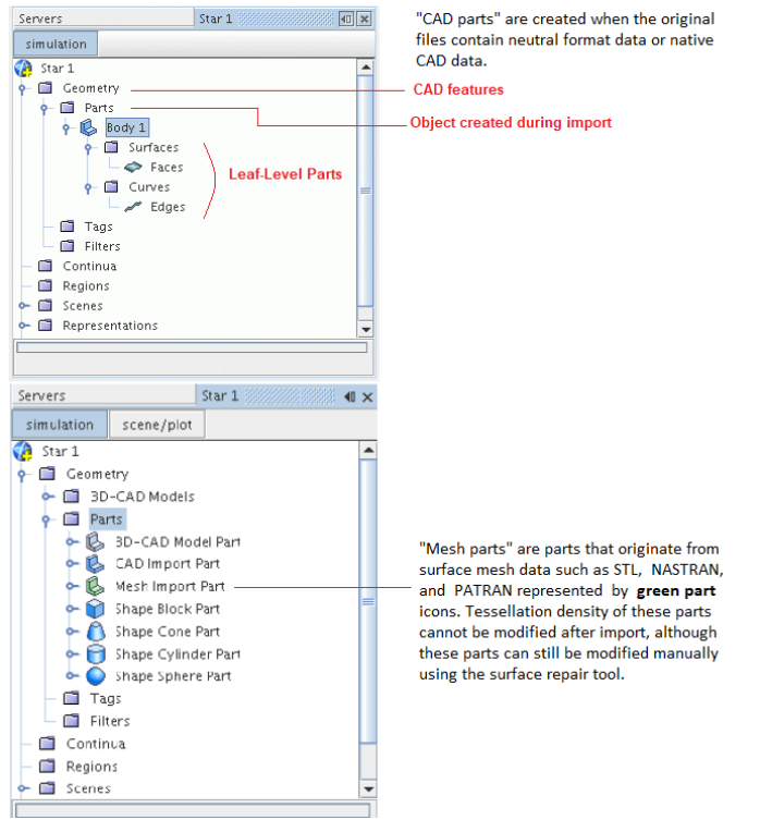
- Parts: There are three different types of part that can be used in a STAR-CCM+ simulation. In 3D case, a part should represent either a solid or fluid volume and not surfaces.
- Geometry parts (model geometry)
- Model parts (including regions, boundaries, and interfaces contained within the Regions, Boundaries, and Interfaces manager nodes - representing the discretized portions of the geometry to be analysed, on which physics models are applied.
- Derived parts (parts used in the definition of analysis reports and for visualizing solution data in scalar and vector scenes.
- Continuum: Continuum is used to contain selections of physics or meshing models that are subsequently applied to one or more regions. Continuum have no geometric definition associated with it.
- Mesh Continuum: A mesh continuum contains a selection of meshing models, such as the surface remesher, the prism layer mesher and the polyhedral mesher. When a mesh continuum is applied to a region, the region is discretized according to the meshing models selected for the mesh continuum. While using "Automated Mesh operation" to generate volume mesh, 'parts' must be assigned to 'regions'.
- Physics Continuum: A physics continuum contains a selection of physics models, such as a chosen flow solver, material models, steady or transient time model, a turbulence model and so on. Each physics continuum represents a single substance that is present in all regions to which the physics continuum applies. Fluid Continuum and Solid Continuum are used to designate Fluid and Solid materials respectively.
Fluids: the colour of fluid nodes change from gray to blue to indicate that fluid models have been activated and continuum is valid.
Solids: the colour of node changes from gray to shaded gray to indicate that models have been activated for this continuum. - Model: Model nodes in the simulation object tree represent simulation features that are active in the current case. Model nodes are contained within the meshing and physics continua to control the construction of surface and volume meshes and physics models to define the behavior of the specified material.
- Regions: Parts are to Geometry as Regions are to Continua. Regions are volume domains (or areas in a two-dimensional case) in space that are completely surrounded by boundaries. They are not necessarily contiguous and can be linked to each other through interface type boundaries. Regions are created either when a volume mesh is imported or when a surface is imported without using geometry parts. Each region is given a unique name during the import process which can be renamed as per user's convenience.
- Boundaries: Boundaries are surfaces (or lines in a two-dimensional case) that completely surround and define a region. Boundaries are never shared between regions - a boundary can belong to only one region.
- Scene: A scene facilitate visual representation of the model. Under a scene, Displayers handle the actual visible objects. Default setups are: Geometry, Mesh, Scalar, Vector and Empty though any scene can use any type of displayer or any mix of displayers. The default scenes just automatically load useful displayers in upon creation. Parts can be added in the properties window after selecting it under the displayer.
| Regions in STAR-CM+ | Parts in STAR-CCM+ |
| Computational domains in STAR-CCM+ are called Region where each region is completely surrounded by boundaries. Boundaries common between two regions can be joined with an interface allowing mass, momentum and energy to pass between the regions. | Parts in STAR-CCM+ are geometrical representation of Objects. Parts can be modified in different ways and used as input for meshing operation and the result of this meshing process gets placed in a region specified in advance. One or several parts can be used as input to one region. Contacts can be created for surfaces common between two parts which are transformed into interfaces when the parts are meshed into regions. |
Following table is an attempt to draw some similarities and analogies between various names and concepts used in CFD programs. However, there is no distinct boundaries and there are overlaps the way these designations refer to underlying objects and collectors.
| Identifier | STAR-CCM+ | FLUENT | CFX | OpenFOAM / ParaView |
| Solvers | Physics Continua | Viscous Model | - | Application |
| Parts | Mesh Continua | Zones | Boundary | |
| Regions | Continua | Cell Zones, Face Zones | Cell Zones, Face Zones | Blocks |
| Domains | Continua | Cell Zones, Face Zones | Cell Zones, Face Zones | Blocks |
| Boundaries | Cell Zones, Face Zones | Face Zones, Edge Zones | Boundary | |
| Zones | Regions, boundaries | Boundary, Patch | ||
| Case | Model | Case | Definition | Folder |
| Scenes | Separate for Geometry, Mesh, Scalar, Vector | Common for Scalar and Vectors, Planes | Common for Scalar and Vectors, Planes | Views and Filters: Render View, Slice View... |
The terms used in this table are building blocks of a simulation which consists of physical space (3D volume designated as domain or region), boundaries of a volume (known as surface regions or face zones), solver types (known as viscous model or continua) and so on. A generic term which can be used for all the objects mentioned in above table is 'collector' which is a collection or group of different physical (nodes, faces...) objects and numerical (turbulence model, material properties ...) objects. Few additional terms used to describe the computational volume are walls, interfaces and contacts.
Excerpts from STAR-CCM+ User Manual: Part-based meshing is a method for generating surface and volume meshes on geometry parts. It is different to region-based meshing in that it uses a series of mesh operations to define the process from the initial geometry to the final volume mesh. Having a series of operations allows you to modify the initial geometry and repeat the entire process with no additional inputs. This makes parts-based meshing particularly suitable for parametric design studies.
Defining the Simulation Topology
Geometry is defined in terms of geometry volume, surfaces, curves and points. The discretized geometry is defined in terms of body points (volumes), faces, edges and nodes / vertices. The collection of these entities are designated as 'parts' in ICEM CFD, zones in "FLUENT", "regions and boundaries" in STAR CCM+ and "Assembly, Primitive 2D, Primitive 3D" in CFX. The computational model to which physics can be applied is defined in terms of regions (domains or zones defined in FLUENT, CFX) and boundaries. Defining the simulation topology is the process of mapping between the geometrical definition of the problem and the computational (or physical) definition.
In STAR CCM+ geometry parts refers to volume which can be assigned to regions, part surfaces can be assigned to boundaries, and part curves can be assigned to objects called feature curves. This mapping is important if all the operations, CAD import till simulation is performed inside STAR-CCM+ environment. If mesh is generated out of STAR-CCM+ environment, these operations need to be performed in that application which will also write output file compatible to STAR-CCM+ requirements. For a typical CFD analysis, simple geometries are usually imported in CAD or non-CAD formats (or in more scientific terms, discrete or tessellated formats), while complex geometries usually come in mixed or hybrid formats, containing both CAD and non-CAD parts.
Difference in Descriptions
Note that there is no UNDO option in general. For example, if you delete a part from model tree, you cannot recover by UNDO operation. There are some UNDO and REDO operations though such as surface repair operations. Most of the programs has keyboard short-cuts like famous control-c and control-v in MS-Windows OS. These are sometimes also called hot-keys. A summary of such keyboard features available in STAR-CCM+ are as follows:
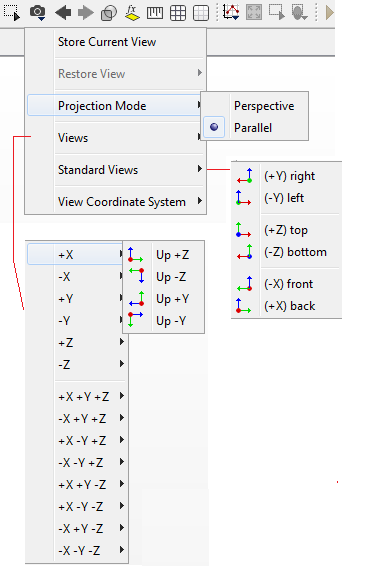
- To align with the X-Y plane, press the 'T' key. Remember 'T' as initial of TOP view
- To align with the Y-Z plane, press the 'F' key. Remember 'F as initial of FRONT view
- To align with the Z-X plane, press the 'S' key. Remember 'S' as initial of SIDE view
- To rotate the model about x-axis, press 'x' key. It will rotate 10° for every press of the 'x' key. Same if true for 'y' and'z' keys
- To fit the view within the Graphics window, press the 'R' key
- To rotate about the selected point, hold down the left mouse button and drag
- To zoom in or out, hold down the middle mouse button and drag
- To translate or pan, hold down the right mouse button and drag
- To rotate around an axis perpendicular to the screen, press the 'Ctrl' key and hold down the left mouse button while dragging
- Double click on an edge and it will attempt to create a closed loop.
STAR-CCM+ Views
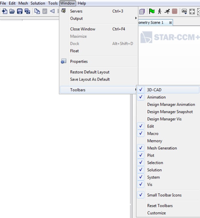
STAR-CCM+ Toolbars
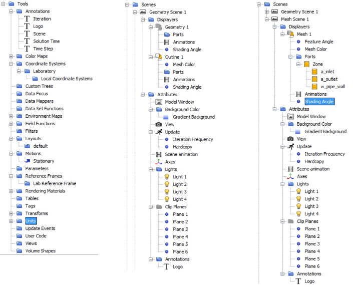
STAR-CCM+ Tools and Scenes
Step-by-Step Approach for Simulations using STAR-CCM+
Step-1: Import Geometry (STEP, Parasolid, STL...) as described here. Uncheck option "Merge Part by Name" to keep parts distinct. Use "One per Surface per Part" to maintain hierarchy defined in input file. Unite bodies which creates a new part and overlapping bodies are merged into single surface: Select bodies > Part Operation > Right click > Boolean > Unite. If the CAD is open sheets, they must be closed to create a part. Use Stitch or Sew tools available in 3D-CAD toolset to connect surface edges. Right-click on the desired surface/stitched body and select Create Part.
Step-2: Before any operation, imprint bodies. Right click Geometry > Operations and select Imprint to connect faces topologically. Repair surfaces as described here. Sometimes tree-structure is deeply nested containing redundant stage(s). Right click Assembly or Composite part under Geometry node and select Explode to move each part or body directly under the assembly. Under 3D-CAD > Body Groups, use Flatten option.
Convert Surfaces to Closed Volumes: if the STEP file contains surface bodies representing a fluid region, select surfaces and use Surface Repair > Stitch. Manually one may use Zip edges (merge two close free edges together within a specified tolerance closing gaps between surfaces), Fill holes and Collapse vertices (to merge a free edge vertex into another vertex, closing small gaps or simplifying geometry - first node select is the target node) to repair the surface geometries. Non-manifold edges (edges shared by more than two faces) is usually repaired by splitting or deleting unnecessary faces.Organize the parts: to rename faces, use "Split by Patch" option under Geometry > Parts > Part Name > Surface Name. Transfer bodies from 3D-CAD to Parts using option "Create Part Contacts from Coincident Entities". Right-click the Parts node under the Geometry node and select "Create Part from CAD Model" to bring it into the simulation context. Geometry > Parts > Part Name > Right click and select "Assign Parts to Regions".
Step-3: Generate Mesh: Follow the method described here. Right click on Geometry &g; Parts > Imported Geometry and select "Create Mesh Operation". Sometimes including "automatic surface repair" while choosing surface remesher helps remove the errors contained in the geometry.
Step-4: Solver Setting: Follow steps described here.
STAR-CCM+ Geometry Import

You can import a surface or volume mesh from an external file via File > Import > Import surface mesh. During geometry import, a choice of centimeters (cm), feet (ft), inches (in), kilometers (km), meters (m) (default), miles (mi), millimeters (mm), micrometers (um) and yards (yd) is allowed. The selection determines the scale factor that is applied to the import surface to make it conform to SI (meters). For example, selecting millimeters automatically scales the vertices by 0.001. If a unit other than one listed was used for the surface file, select the meters option (equivalent to no scaling). After the import process is complete, you can apply a user-defined scaling factor to scale the mesh.
If a unit other than meters (m) was selected, then the option to Set preferred units for length is available (off by default). This option can be used to set the selected unit as the default for all mesh reference and input values that involve length. Leaving the option off maintains meters as the default unit for length.
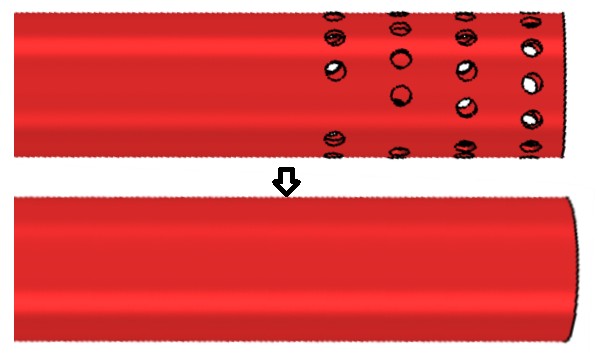
Manual Surface Preparation
An imported geometry can be of poor quality to properly mesh and achieve a useful simulation result. The geometry may be self-intersecting, it may have gaps, there may be free edges or non-manifold vertices. The manual surface preparation tools contained within STAR-CCM+ allow you to:- diagnose and locate each surface issue
- delete faces and edges and create new ones
- collapse and smooth vertices
- fill and patch holes
- split and swap edges
- locally zip edges
- locally remesh faces (with or without feature retention)
- isolate connected surfaces and delete them if necessary
- inflate thin shell/baffle surfaces so that they have thickness
- translate a surface
Convert sheet bodies to solids: reference community.sw.siemens.com
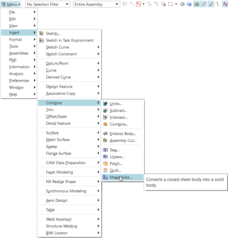
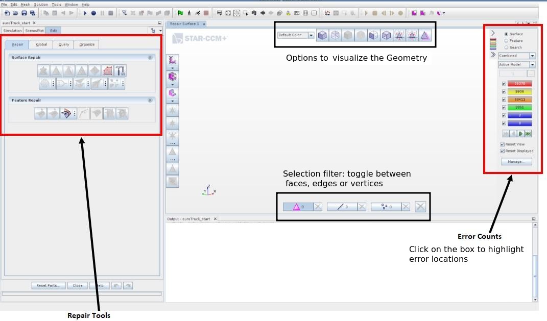
Surface Repair Tool: Surface repair is accessed by right-clicking on the part and selecting Repair surface option.
This is a utility that allows to directly repair the part surface. It is easy to use and will highlight each error. But in case any geometry upstream needs to be changed, one need to redo the repair manually, as it is not a pipelined operation. This utility is a good place to start after importing the geometry as it will show how many errors must be fixed and where they are and what type they are.
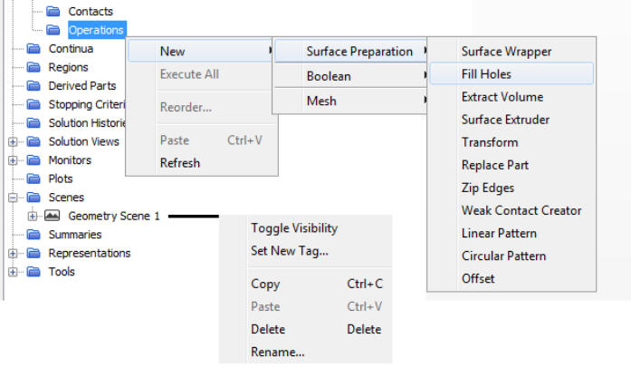
Fill holes is an operation for preparing a geometry for an internal flow simulation by doing what the name suggests: capping and filling holes in the part. This is possible in 3D-CAD and the surface repair tool, but this operation lets you add it to an automated pipeline. Note there is no Apply button. First select the closed loop (manually or double click on one the edge elements) and then click the fill hole button.
Extract volume pulls an internal volume from a part, typically after Fill Holes or similar operation has been used to cap the openings to prepare the geometry for an internal flow simulation.
One of the most useful operations is that to replace a part. This operation makes swapping out a geometry part repeatable and traceable, unlike manually replacing the part by right clicking it in the tree.
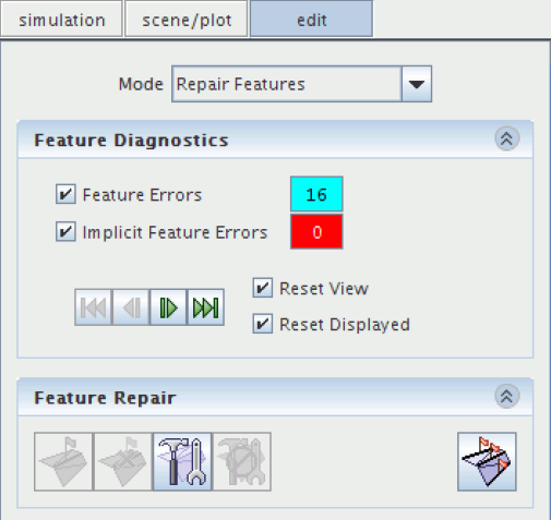
Repairing Features: All feature curves that are required to represent the geometry needs to be correctly identified in the surface mesh. This process identifies feature errors - that is, edges that are features but are not represented as such, and edges that are incorrectly represented as features. Feature curves indicate where sharp edges exist and are listed under the Feature Curves node for each region. If the surface remesher operation is performed to improve the surface mesh quality, then including feature curves is necessary to preserve sharp edges and surface detail (such as imprints). If the feature curves are not included, then edges are rounded off and surface detail is lost.
Closing Gaps: Project vertices onto a set of faces to close a gap using "project selected vertices tool".
Duplicate Faces -- surface repair -- Merge/Imprint: The tool also lets you merge two or more overlapping (co-planar) surfaces or sets of faces. When using Merge/Imprint on a single part, the result is either a common shared surface or no surface at all (that is, the common area is removed). If there are multiple parts, the tool creates part contacts for the shared surface. Similarly, for feature curves belonging to the same parts, the tool can imprint two or more edges onto each other, effectively zipping them together. You can also imprint edges onto faces and imprint faces onto edges, depending on the requirement. No edge options are available when imprinting across multiple parts. In all instances, the faces or edges do not need to belong to a closed surface in order to use the tool.
Automatic repair tool can fix certain global surface problems that relate to bad quality, close proximity and/or intersections (pierced faces) at the push of a button. If you want to fill a large number of holes automatically or zip a large number of edges then you should use the hole filler and edge zipper tools respectively.
STAR-CCM+ includes a comprehensive set of surface-repair tools that allow users to interactively enhance the quality of imported or wrapped surfaces, offering the choice of a completely automatic repair, user control, or a combination of both. One of the most important elements of surface repair tool is its diagnostics tool. It offers functionality to identify error prone parts, surfaces and feature edges and provide real time information via the browse tool as you fix them.
Two defeature modes [accessed by right-clicking the body] are available in STAR.
- Automatic mode is applicable to Bodies and automatically defeatures fillets, chamfers and holes based on a user-defined criterion.
- Manual defeature mode is applicable on Faces and is used to delete and heal user-selected faces. From V2020.2 onwards, the feature Delete Interior Faces deletes all faces that exist between the two faces selected by the user.
Non-conformal Imprinting
During the process of non-conformal imprinting, pairs of split surfaces are created on contacting parts without altering the individual parts or creating shared faces. To achieve a non-conformal mesh when imprinting these surfaces, before you imprint the parts, activate Show Advanced Parameters and set Resulting Mesh Type to Non-Conformal. After imprinting the parts, the resultant surfaces are non-conformal, which means that the surface discretization on the imprinted surfaces does not match. Each part remains separate and there is no shared surface between each part. However, the original discretized surfaces are cut and a pair of split part surfaces are created which represent an in-place part contact between the surfaces.Mesh Generation in STAR-CCM+
Excerpts from user manuals and tutorials for STAR-CCM+STAR-CCM+ offers 7 types of meshing models: [1] Tetrahedral - tetrahedral cell shape based core mesh, [2] Polyhedral* - arbitrary polyhedral cell shape based core mesh, [3] Trimmed - trimmed (Cartesian or cut-and-cell or snappyHexMesh) hexahedral cell shape based core mesh, [4] Thin Mesh - tetrahedral or polyhedral based prismatic thin mesh, [5] Extrduder Mesher, [6] Prism Layer Mesher and [7] Advancing Layer Mesh - polyhedral core mesh, with in-built prismatic layers that advance inward from a polygonal surface mesh.
*In STAR-CCM+, a special dualization scheme is used to create the polyhedral mesh from an underlying tetrahedral mesh, which is automatically created as part of the process. The polyhedral cells that are created typically have an average of 14 cell faces.Local Refinement
Excerts from User Guide: "Volumetric controls in the shapes of bricks (cuboids), spheres, cylinders, and cones can be used during the volume meshing of the core mesh to increase or decrease the local cell density. Arbitrary shaped volumes that are imported as parts can also be used to define the refinement volume. Feature refinement is automatically included in the case of the trimmer meshing model."
There are two meshing approach in STAR: parts-based meshing and region-based meshing. Parts-based meshing approach is recommended, though one need not always follow this approach to generate a mesh. For simple geometry and assemblies consisting of few sub-assemblies, one can import parts, assign parts to regions, then generate mesh at the regions level. However, if while working with assemblies that contain tens or hundreds of parts, parts-based meshing approach is recommended.
There is an option to use Automatic Surface Repair during Surface Remesher operation. This can help repair small errors in the surface, although it is not recommended for multi-volume models. Automatic Surface Repair cannot repair non-manifold edges or vertices or correct free edges.
Excerpts from User Guide: Parts-based meshing detaches the meshing process from physics modelling and provides a flexible and repeatable sequence of mesh operations. The sequence of mesh operations is called the meshing pipeline.
To capture the complex and intricate features of the geometry the mesh generation process utilizes contact prevention conditions, volumetric controls and the wrapper scale factor. Wrapped surface is then re-triangulated using the surface remesher.
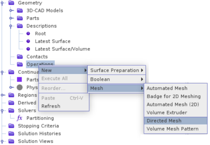
Directed meshing or swept meshing: Directed meshing allows you to generate a high-quality structured mesh by creating quadrilateral elements on a surface of a body and then sweeping them through its volume. It requires a Source Face, a Target Face, and the guide face along which the directed mesh is swept. A directed mesh is a Parts Based Meshing Operation. Identify the source and target faces. Highlight the source face and Right-click > Add to Source. Repeat for target face to Add to Target. Next, set up a new source mesh. Right-click Source Meshes > New Source Mesh > Patch Mesh. This brings up the patch mesh editor. Select the edges (feature curves) of the source face to generate quad elements as per desired refinement.
Once surface mesh on source face is ready, to create the volume distribution, Right-click Mesh Distributions > New Volume Distribution. In the Properties window for the volume mesh, set the number of layers to required refinement in sweep direction and then right-click Directed Mesh > Execute.
Generate and Display a Mesh
To generate a mesh: Right-click Geometry -> Operations and select New -> Automated Mesh. In the Create Automated Mesh Operation dialogue: Select the zones or volumes from the Parts list. To specify the mesh settings: Right-click the Geometry -> Operations -> Automated Mesh -> Default Controls node and select Edit.... In the Default Controls dialogue, set the desired parameters such as Base Size, Number of Prism Layers, Surface Curvature, Surface Proximity... To customize the mesh to modify the mesh settings only on specific surfaces: Right-click the Geometry -> Operations -> Automated Mesh -> Custom Controls node and select New -> Surface Control -> Right-click the Custom Controls -> Surface Control node and select Edit -> Update Minimum Surface Size and tick 'Disable' under Prism Layers.To display the mesh: Select the Scenes -> Geometry Scene 1 -> Displayers -> Geometry 1 node. In the properties window, activate (tick checkbox) Mesh to display the surface of the mesh. Right-click an empty part in the geometry display graphics area and select Apply Representation -> Volume Mesh.
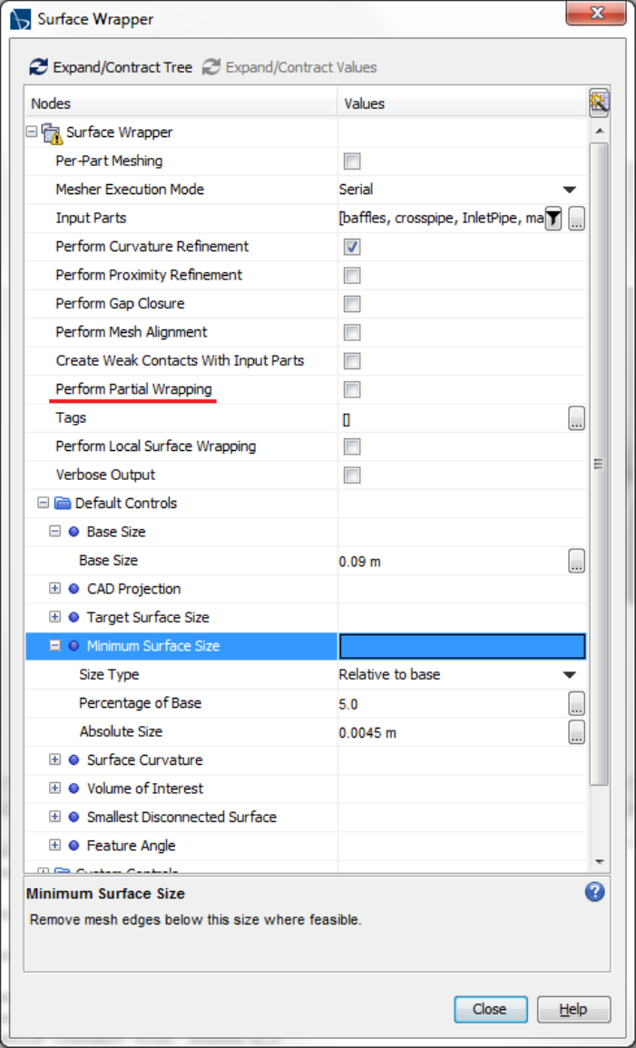
Surface wrapping and partial wrapping: In addition to refining the surfaces of parts in the wrap, partial wrapping can be used to exclude selected parts or part surfaces from the wrap operation. Excluded parts from the wrap, the original tessellation of the those parts is passed through to the final wrap surface. Some geometries only require surface wrapping for a portion of their surface. The surface wrapper allows you to exclude part surfaces that you consider sufficiently well tessellated for subsequent mesh operations. In some cases wrapping the whole geometry is unnecessary and can defeature highly detailed part surfaces unless the surface wrapper is excessively refined using custom controls and contact preventions. Select the Geometry > Operations > Surface Wrapper node and activate the "Perform Partial Wrapping".
Per-part meshing feature of "surface wrapping" operation allows multiple disconnected parts to be wrapped separately. The Minimum Size value indicates the triangle size in the space between the two parts, which determines the octree refinement in the area. The value should be set smaller than the gap size (typically one half or one quarter of the distance). It is just a stopping size for the surface wrapper refinement, which results in the two surfaces being separated.
Surface wrapping process steps:
- Global surface wrap at part / component level: Right-click the Geometry > Operations node and select New >> Surface Wrapper. In the Create Surface Wrapper Auto Mesh Operation dialogue, select appropriate part/assembly. Expand the Surface Wrapper > Default Controls node and set Base Size, Minimum Surface Size and Volume of Interest.
- Refining the Mesh on Part Curves: To make sure that you capture the detailed features in the surface mesh, apply mesh refinement to all the part curves. To apply refinement to all part curves: Right-click the Surface Wrapper > Custom Controls node and select Ne>> Curve Control. STAR-CCM+ adds a curve control node within the Custom Controls node.
- Preventing Contact between Close Surfaces: To make sure that these two surfaces do not touch each other in the wrapped surface, apply a contact prevention between the nose and main body. To apply contact prevention: Right-click the Operations > Surface Wrapper > Contact Prevention node and select New > One Group Contact Prevention Set. Contact prevention for small clearances -> One Group Contact Prevention Set / Two Group Contact Prevention Set
- Local refinements near gaps using "Surface Control"
- Perform "partial wrapping" to capture local features like baffles, channels...[Split surface by patches, Preserved Input Surfaces-> Select "Excluded Surfaces"]
- Creating the Fluid Volume: The fluid simulation requires a volume mesh between the walls of the simulation domain. To create the part that defines the outer surface of the volume mesh, subtract the output of the surface wrapper operation from the bounding box. Right-click the Geometry > Operations node and select New > Subtract. In the Create Subtract Operation dialog, select Bounding Box and Surface Wrapper, then click OK. A Subtract node appears beneath the Operations node, and a Subtract part appears beneath the Parts node.
Contact Prevention
When the clearance between two surfaces is less than the target surface size, use a contact prevention to tell the wrapper not to join the two boundaries. The Minimum Size value indicates the triangle size in the space between the two parts, which determines the Octree refinement in the area. The value is smaller than the gap size (typically one half or one quarter of the distance). You can still join the surfaces even though a Minimum Size value is set. The Minimum Size value is simply a stopping size for the surface wrapper refinement, which results in the two surfaces being separated. The value also has to be greater than zero.Mesh Interfaces
There are two categories of interfaces in STAR-CCM+ and any interfaces that are created during the simulation setup process are accessible via the Interfaces manager node. The Interfaces node has properties and a pop-up menu.
- between boundary faces: this include contact interfaces between solid and fluid regions, internal interfaces between fluid regions and baffle interfaces representing thin-walled separators. There are two categories for interfaces between boundaries:
- Direct Interface - boundary faces are intersected or imprinted resulting in conformal mesh: Baffle, Porous-baffle, Contact, Fa, Fluid Film, Fully developed, Internal
- Indirect Interface - boundary faces are coupled using mapping or mixing: Mapped Contact, Mixing Plane Interface, Blower Interface
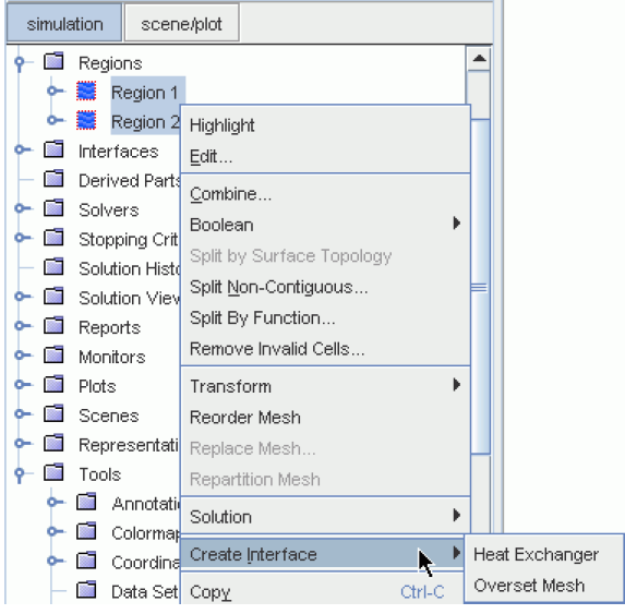
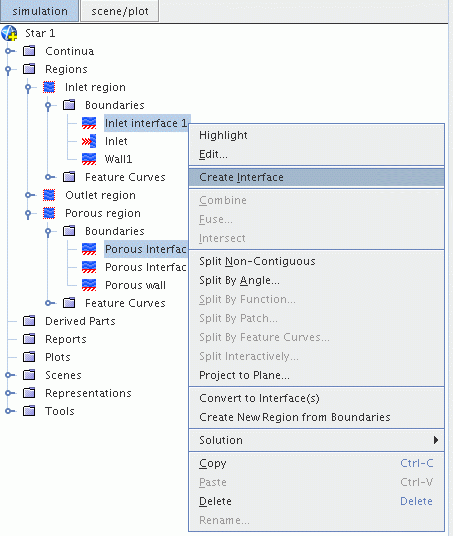
- between region volumes: Interfaces are created between region volumes to set up an overset mesh or to model heat transfer in a dual stream heat exchanger. To create an interface between regions ➛ Select the two regions that define the interface (press and hold the Ctrl key to select the second node) ➛ Right-click and select the Create Interface pop-up menu item, and make a selection from one of the options in the submenu.
Interface Types determines the behavior of the interface with respect to the modelling of flow and heat transfer. Interfaces can connect individual boundaries (faces) or entire regions (volumes). Following interface types and connectivity are available in STAR-CCM+
| Type | Connects to | Topology | Connectivity |
| Baffle | Boundaries | Direct Interface | Imprinted |
| Porous Baffle | Boundaries | Direct Interface | Imprinted |
| Contact | Boundaries | Direct Interface | Imprinted |
| Fan | Boundaries | Direct Interface | Imprinted |
| Fluid Film | Boundaries | Direct Interface | Imprinted |
| Fully Developed | Boundaries | Direct Interface | Imprinted |
| Internal | Boundaries | Direct Interface | Imprinted |
| Mapped Contact | Boundaries | Indirect Interface | Mapped |
| Mixing Plane | Boundaries | Indirect Interface | Connect Average |
| Blower | Boundaries | Indirect Interface | Connect Average |
| Heat Exchanger | Regions | Heat Exchanger Topology | Modeled |
| Overset Mesh | Regions | Overset Mesh Topology | Modeled |
Note that "creating an interface" is not same as "converting boundaries to an interface". While "converting boundaries to an interface" single and usually common boundary belonging to a surface mesh is duplicated and then an interface made between the original and the copy for the primary purpose of defining multiple regions for meshing. To create an interface between boundaries, select the two boundaries that define the interface. The first boundary selected is termed the master boundary and the second is called the slave boundary.
Imprint is a process of making a common boundary between two volumes. If two square blocks are touching each other, there are two faces, one each belong to each square. When imprint is performed, the one of the common surface is deleted. The imprint operation will result into entity known as 'contacts' in STAR, and may become interfaces when parts are transferred to regions. Four types of contact definition exists: In-place, Weak in-place (meshed non-conformally), Periodic, Baffle. Part-part contacts may be created (a) automatically during geometry import, (b)by imprinting, (c)by tolerance based searching and (d)manually. STAR-CCM+ allows to imprint parts non-conformally. This process is useful when:
- a conformal interface is not necessary to achieve solution accuracy
- there are many contacting parts
- each part is within many pairs
- there are gaps between the CAD parts
STAR-CCM+ Mesh Checker
When a mesh created in external application is imported into STAR, by default unit of [m] is assigned to the dimensions of the mesh. Hence, the imported mesh needs to be scaled appropriately. Mesh > Diagnostics... menu option can be used to generate Compact and Full report summarizing the entity count, mesh extents and mesh quality.Mesh Diagnostics: Compact
The compact report for a volume mesh generates statistics for each mesh region having following sub-sections: Entity count, Mesh extents, Mesh validity check, Face validity statistics and Volume change statistics.
Mesh Diagnostics: Full
The full diagnostics report is structured in a similar way to the compact report and contains all the information the compact report produces with following extra items for each region and the overall summary: Boundary details, Entity count per cell shape, Volume range (the minimum and the maximum volumes of an element in entire domain), Maximum interior skewness angle. The boundary details are split up as Number of faces, Boundary extent, Surface area and Maximum boundary skewness angle. To check if the volume mesh has zero or negative volume cells, either run the mesh diagnostics report or initialize the solution. Cells having ≥ 0 volumes can be identified and visualized using threshold values.
The first section of the report contains summary of all regions in the format: region_name (index 235): X cells, y faces, z vertices. The next section gives detail information for each region starting with statement "---- Computing Statistics in Region: region_name". For each region, following parameters are reported:- ENTITY COUNT: number of cells, faces, vertices and edges
- EXTENTS: diagonal of bounding box
- MESH VALIDITY: confirming that there is no negative volume
- FACE VALIDITY STATISTICS: value reported in 8 intervals starting with < 0.5, 0.5 ~ 0.6 ... >1.0
- VOLUME CHANGE STATISTICS: value reported in 8 intervals.
Mesh Quality Checks in STAR-CCM+
Face quality is a measure of similarity between a face and the ideal face shape which is an equilateral triangle. The surface diagnostics calculate face quality = "in-circle radius / circumcircle radius" x 2. For an equilateral triangle, in-circle radius * 2 = circumcircle radius. Thus, face quality '0' is degenerate triangle and 1 is the ideal shape. Default value of poor element setting in STAR-CCM+ is 0.01. The other definition in STAR-CCM+ as used in Surface Remesher is that quality of a triangle = the ratio of the triangle face area to the area of an equilateral triangle that would exactly fit inside the circumcircle of the triangle. The default value for surface remesher is 0.05
Dihedral angle of an edge is the angle between its adjacent faces. Edges are considered invalid if they are free or non-manifold as a dihedral angle cannot be calculated for such edges.
- Polyhedral quality: This value refers to the cell quality of the polyhedral cells.
- Cell face validity: This value refers to the face validity of the cells.
- Cell orthogonality: This value refers to the angle between the normals of two faces in a cell that share an edge. The closer the cell edge angles are to 90 degrees, the more orthogonal the cell is.
- Cell skewness angle: This skewness measure is designed to reflect whether the cells on either side of a face are formed in such a way as to permit diffusion of quantities without these quantities becoming unbounded. The skewness angle the angle between the face area vector (face normal) and the vector connecting the two cell centroids. Skewness angle = 0 indicates a perfectly orthogonal mesh. Variables that are stored at interior faces in STAR-CCM+ cannot be displayed and hence the worst skewness angle for all the faces of a cell are stored in that cell. Thus, two cells often have the same skewness angle corresponding to the face that they share. To reduce the impact on robustness, avoid skewness angles greater than 85° as reported in the mesh diagnostics full report.
- Cell Quality: It describes relative geometric distribution of the cell centroids of the face neighbor cells and of the orientation of the cell faces which is specified as 'Orthogonality' in some programs such as ANSYS FLUENT. Generally, flat cells with highly non-orthogonal faces have a low cell quality. A cell with a quality of 1.0 is considered perfect.
- Cell volume ratio: This value refers to the volume change between neighboring cells.
- Boundary Skewness Angle: it is defined as the angle between the area vector and the vector connecting the cell centroid and the boundary face centroid. This angle is important since the dot product of these two vectors appears in a denominator in a component of the equation for diffusive fluxes at a boundary face. In turbulent flows where wall functions are used, the equation for diffusive fluxes at a boundary is not used to compute diffusion fluxes at walls, so boundary face skewness become less important. However, it is important for laminar flows and for heat transfer in solids. To reduce the impact on robustness, avoid boundary skewness angles greater than 85° as reported in the mesh diagnostics full report.
- Face Validity Cell Metric: It is an area-weighted measure of the correctness of the face normals relative to their attached cell centroid. A face validity of 1.0 means that all face normals are correctly pointing away from the cell centroid. Values < 1.0 mean that some of the cell faces have normals pointing inward towards the cell centroid indicating some form of concavity. Values < 0.5 signify a negative volume cell.
- Volume change metric: It describes the ratio of the volume of a cell to that of its largest neighbor. A value of 1.0 indicates that the cell has a volume equal to or higher than its neighbors. A large jump in volume from one cell to another can cause potential inaccuracies and instability in the solvers. Consider cells with a volume change value < 10-5 to be suspect and investigate these cells further.
Removing Invalid Cells tool allows to remove mesh cells from the volume mesh region definition based on one or more of the following 4 mesh criteria: Face Validity, Cell Quality, Volume Change and Contiguous Cells. STAR-CCM+ moves all the removed cells into a separate region that is not used in the analysis. Symmetry plane boundaries are automatically added to the neighboring cell faces of cells that have been removed, minimizing the impact of these removed areas on the solution. Cells that do not meet the provided criteria are moved into a new region called Cells deleted from [Region] where [Region] is the name of continuum which these deleted cells belong to.
- pierced faces: A pierced face is one that has one or more edges of another surface cell piercing it.

- close proximity faces (surface folds and overlaps):
- free edges (holes and mismatched edges): Free edges refer to cell faces that are not connected to a neighboring face. free edges can be fixed by using the hole filler, the edge zipper, or the manual fixing tools, depending the nature of the problem. To repair click on the number on the Count list and all the problematic part would appear in pink. Then if it is for example problematic faces (that are over created) select them one by one or with ctrl or with the Zone selection tool and delete them. Then you will have to fill the holes you created with this action or the ones made by the software when importing the geometry.
- non-manifold edges: A non-manifold edge refers to a cell face edge that is connected to two (or more) other edges. A non-manifold edge is sometimes valid depending on whether the surface cells causing the problem are supposed to be a part of the geometry or not. For example, consider a geometry that contains a baffle surface that is joined to the exterior surface. This geometry is not a problem as long as the surface is converted to an interface before proceeding with the volume meshing. If the non-manifold edge is not expected, then you can delete the faces that are causing the problem.
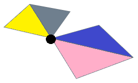
- non-manifold vertices: Typically vertices connected to a surface instead of two or more edges.
- holes or leaks: Leaks are not desired because they cause an inversion in the wrapping process, which results in the incorrect volumes being wrapped. Run the leak detection tool to identify less obvious gaps and holes. The hole filler can be used to close any closed loop (both single and multiple loops) planar hole within a surface. The edge zipper can be used to join two mismatched surface edges that are within close proximity to one another, so that a closed surface is formed. Two different tools are available to help close off holes, namely the polygonal patch fill and the hole filler.
The polygonal patch filler is a quick and easy way of closing arbitrary shaped holes which do not have a closed loop definition and/or are not planar. The process literally 'patches' up the surface by creating faces that cover the hole area completely. Having an overlap in the patched surface is perfectly acceptable as the wrapper deals with this overlap automatically.
- The hole filler is a more exact method of filling well-defined holes by using a closed loop feature edge definition around the hole.
- missing faces: This refers to open cells where 1 or more faces are missing and elements need to be created to make a valid 3D cell
Compute Volumes: Right click on 'Reports' in the simulation tree and selecting New Report > User > Sum. To compute the volume, select 'Volume' as the scalar field function and the Volume Mesh as the representation. Further, only the (3D) region of interest needs to be selected under parts and not its boundaries. When a boundary is selected, the report includes the volume of those cells that touch the surface. This can result in double counting of cells in the report resulting in a value larger than the actual volume.
Replace parts: "Operations > New > Surface Preparation > Part Replace". Changing the input automatically updates the workflow.
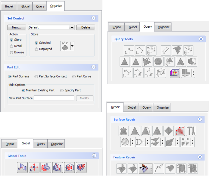
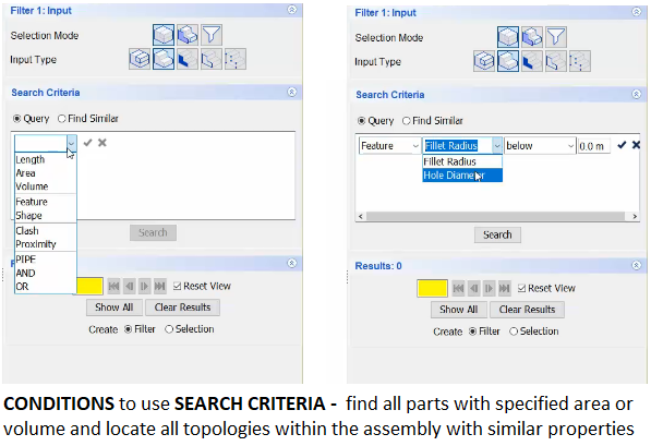
Filters
Six basic repair filter types (or predicates) available to use are listed below. Filter predicates can be used individually to search for parts or pieces of geometry and/or can be compounded within a filter, using logical operators (AND, OR or PIPE) to provide additional control.- Part Name: Search for parts based on the presentation name
- Part Surface Name: Search for part surfaces based on the presentation name
- Area: Search for faces/surfaces based on the area
- Volume: Search for closed surfaces based on the volume
- Area/Volume Ratio: Search for closed surfaces based on the area/volume ratio
- Face Count: Search for faces/surfaces based on the face count
Continua: Solver Setting
Excerpts from User Guide: Assigning parts to regions creates a relationship between the meshed part and the physics region where part-level objects (parts, part surfaces, and part curves) are associated to their equivalent region-level objects (regions, boundaries, and feature curves). This action allows STAR-CCM+ to convert the volume mesh to a finite volume representation that the solver can use to obtain a solution. These assignments do not need to be one-to-one. That is, you can assign multiple part-level objects to the same region-level objects.
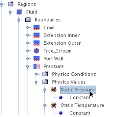
Set Boundary Conditions

File Auto Save in STAR-CCM+
For transient simulations as well as steady state simulations, intermediate bak-up results files need to be created and monitored. To set auto-save option: Main Menu > File > Auto Save: Under "Max Autosaved Files" set it 10. Under the node Update, tick Enbaled and update field appropriately.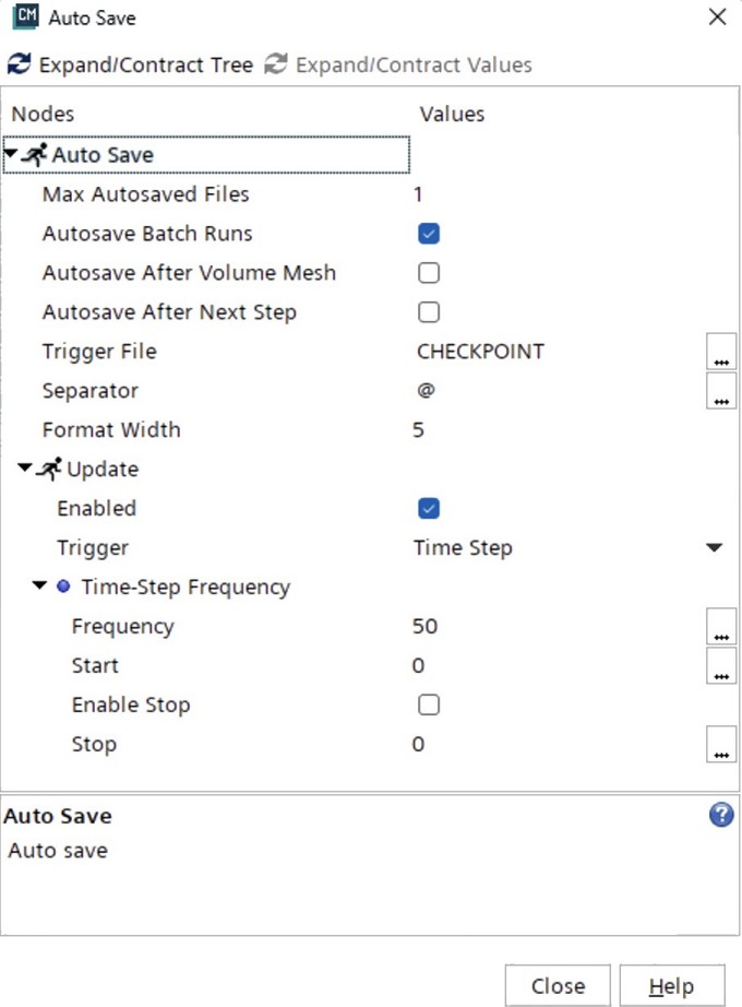
Create Monitors in STAR-CCM+
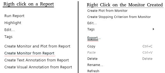
Monitors such as heat balance of pressure drop between inlet to outlet are recommended to monitor for convergence. If reports named "Pressure Inlet", "Pressure Outlet", "HTR_Hot" and "HTR_Cold" are created, corresponding field functions are generated for each report, allowing to be used in an expression. Create an Expression report -> Rename this report to "Heat Balance" -> Click (Custom Editor) in the Definition property -> In the "Heat Balance" - Definition dialog, enter (${HTR_HotReport} - ${HTR_ColdReport}) -> Right-click the "Heat Balance" node and select Create Monitor and Plot from Report. To be able to visualize the cells with high residuals, enable the option "Temporary Storage Retained" for the solver under 'Properties' window.
Reports > System
- Steady State Simulations
- Solver Iteration CPU Time: Reports the CPU time of last iteration
- Solver Iteration Elapsed Time: Reports the Elapsde Time of Last Iteration
- Total Solver CPU Time*: Cumulative CPU Time Report
- Total Solver Elapsed Time: Cumulative Elapsed Time Report
- Physics Continuum Iteration: Current iteration number for the selected Physics Continuum
- Transient Simulations: in addition to above reports, following are available:
- Solver CPU Time per Time Step
- Solver Elasped Time per Time Step
- Physics Continuum Physical Time: Current physical time for the selected Physics Continuum
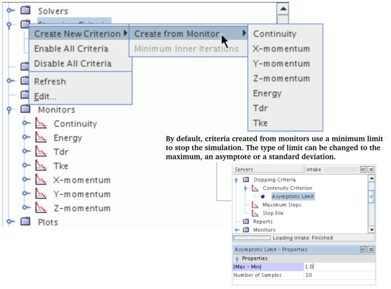
Stopping Criteria in STAR-CCM+
Automatically generated stopping criteria cannot be deleted, but the Enabled property can be activated or deactivated.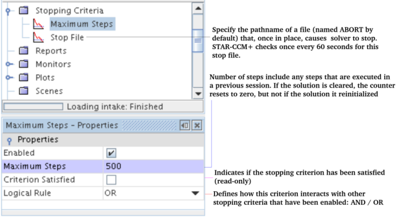
Save images on remote HPC cluster/server: Under the 'Scene' tab, there is option Update. Activate save picture to save the Scene at specified iterations or intervals.
Transient Tables in STAR: The variable name can contain a units specification. The units are specified within a set of parentheses () as part of the variable name:
"Time (s), "Temperature (C)"
0, 25
2, 50
5, 75
Multiphase Flows in STAR-CCM+
To enable multiphase settings in STAR-CCM+ the order of selection is important: Three-dimensional > Steady > Multiphase > Eulerian Multiphase (EMP) > Turbulent > Gravity. To create the Phase Interaction, select the continuous phase first. Phase interaction type can be specified by selecting the dispersed phase.To improve convergence behaviour: turn-off secondary gradients through right click on Models > Eulerian Multiphase (EMP) node. In STAR, it is common practice to use density of continuous phase as reference density.
Domain or region specific initialization: Regions > Region Name > Physics Conditions > Initial Condition Option > Chose "Specify Region Values" from drop down where "Use Continuum Value" is specified.
Troubleshooting divergence for Eulerian Multiphase (EMP): Turn off secondary physics initially by starting with laminar. Volume fraction equations are generally the main source of divergence. Use small under-relaxation factors (0.2 or lower for volume fraction). Use coupled flow solver instead of segregated. EMP is very sensitive to mesh issues - keep aspect ratio ≥ 10 and (though counter-intuitive) fine mesh may initially not converge. If possible, run single-phase solution first and then switch to multiphase. EMP simulations behave better in transient mode which can be run for small duration to develop initial field. Liquid jets into air is an example of strong pressure–velocity coupling due to high density ratio of water and air. The option to gradually increase the density of liquid phase may work in some cases.
Field Functions in STAR-CCM+
Field functions are mathematical expressions to define boundary conditions, material properties and booleans. Few basic rules that applies to creating Field Functions in STAR are described below.- The name of field functions can contain few special characters: For example 'Split@X=0.50[m]' is a valid name.
- If the name contains any non-alphanumeric characters other than underscore '_', enclose the field function name in curly braces, '{...}' such as ${Split@X=0.50[m]} or ${test-Temperature}.
- Creating Field Function Expressions: color code to guide the editing process
- Green indicates a syntactically correct reference to an existing field function
- Parentheses appear in yellow to indicate the matching parenthesis
- Red indicates an incorrect entry
- If a field function reference has red text (but no black text or red background) the color represents a syntactically correct reference to a field function that does not yet exist
- Field function definitions are always done in SI units, independent of the units that you use for input or display.
- Scalars are defined with single $ such as $Pressure or $Time and vectors with $$ such as $$Position and $$Velocity
- Field function names are case-sensitive. Thus, $Time and $time or $Radius and $radius are not same. Since the names are case-sensitive, they must be entered in the field function definition exactly as they are shown in the function name. {$Time} has unit of seconds, ${TimeLevel} is a counter like iteration number which keeps track of time-history of the solution (the current time step, previous time step, previous to previous time step and so on).
- Field functions access data on specific parts that are defined in the simulation
- Field functions used to define expressions cannot be a function of space that is (x, y, z). They must evaluate to a single number as the expressions are constants in space. Variables such as $Time, $TimeStep, and $Iteration are valid where as variables such as $Temperature or $Pressure are not valid as they have different values at every point in space and hence cannot be used in expressions.
- Literal constants can have a unit specification in a different system and are parsed at run time. The syntax for the units is <number units>. For example: <0.001 kg/m/s>, <10 psi>, <0.05 lb/ft^3> The character hyphen "-" binds tighter than "/", so kg/m-s^2 equals (kg)/(m-s^2) not (kg/m)*(s^2).
- When defining an expression or a field function that reference other field functions within it, prefixed that Field Function with $, such as $vol_flow_rate.
- Components of vectors are retrieved by adding additional $ such $$Velocity[0], $$Velocity[1] and $$Velocity[2] refer to X-, Y- and Z-components of the velocity vector. Subscript operator [] is appended to access components of the vector with indices of [0], [1], or [2].
- $$Position(@CoordinateSystem("CylCS"))[0] - The components of a local cylindrical coordinate system is defined by @CoordinateSystem(<Name of Coordinate System>) where <Name of Coordiante System> = "CylCS" in this example. Note that $$Position[0], $$Position[1] and $$Position[2] refer to r, θ and z axes respectively.
- When field functions are accessed on boundary parts, following rules by default: 1) If the data is stored on the boundary, the boundary data are accessed. For example "wall velocity" values stored in wall boundaries. 2)If the data is not stored on the boundary, the cell data from the cells in the region adjacent to selected boundary are accessed. For example, wall-adjacent fluid velocity are stored in the cells.
- When Ignore Boundary Values option is switched ON, the field function is evaluated from the data stored for cell next to the boundary.
- To define a vector, array or position field function in terms of its components, specify the 3 components inside square brackets separated by commas: [($$Centroid[0] <= 1.0) ? 2.5 : 0.0, 0.0, 5.0]
- Initialize a particular volume: $${Position}[0] >= 0.50 && $${Position}[1] <= 1.00 && $${Position}[0] <= 2.50 && $${Position}[1] >= 0.25 ? 300 : 323 - this sets temperature in a cuboid to 323 [K]. To initialize a field variable in spherical volume: $$Position( @CoordinateSystem( "Laboratory.spheric" ) ) <= 0.50 ? 323 : 300. This is equivalent to: if($$Position( @CoordinateSystem( "Laboratory.spheric" ) ) <= 0.50, 323, 300).
- Set transient boundary condition where temperature ramps up linearly from 300 [K] to a value of 500 [K] at a time of 5 [s]. ($Time >= 5.0) ? 500 : 300 + (500 - 300)/5.0*$Time. This is short form of conditional IF-ELSE statement. Ternary operator "? :" defines a condition operation similar to the C language.
- Divergence of velocity ∇.v = div($$Velocity), Divergence of density, velocity ∇.ρv is specified as: div($Density * $$Velocity), Gradient of pressure ∇p is specified as: grad($Pressure), Curl of velocity ∇×v is specified as: curl($$Velocity).
- Pressure ratio to get pressure in atmosphere [atm] unit: ${AbsolutePressure}/101325.0. Note that the default pressure option in Star CCM+ is given as absolute pressure rather than the relative pressure.
- User field functions can be previewed by without actually running the simulation. The output values for the dependent variable is calculated by substituting the values of each of the independent variables and sweeping through the specified range.
- The dot product can be used to find components of a vector where unit($$Area))*unit($$Area) is used to define unit vector for area. For example, normal component of wall shear stress: sN = dot($$WallShearStress, unit($$Area)) * unit($$Area). Since, $WallShearStress is a vector sum of normal and tangential shear stresses, sT = $$WallShearStress - $$sT
- Multiple if conditions - Split a region (Split Regions by Function dialog) into 3 parts: ($$)Position[1] <= 2.5) ? 1 : (($$Position[1] >= 0.5) ? 2 : 0). In this case, after the split: The cells where 0.5 < y < 2.5 belong to Region 1, as the field function does not affect them. The cells where y ≤ 0.5 belong to Region 1 2, as it is the created region with the least cells. The cells where y ≥ 2.5 belong to Region 1 3, as it is the created region with the most cells.
- stepFun = ($$Centroid[2] <= 50) ? 0 : 1 - this creates a step function at the global z-coordinate of centroids of cell ≤ 50
- Field function for temperature dependent thermal conductivity: thCondAir = 1.52e-11 * pow($Temperature,3) - 4.86e-8 * pow($Temperature,2) + 1.02e-4 * $Temperature - 3.93e-4 where T is in [K]. As per the formulat, thCondAir = 0.0262 [W/m-K] at T = 300 [K].
- In Simcenter STAR-CCM+, collocated values refer to field values like temperature or pressure, that are defined at the same physical location (cell center) as the mesh cells. For example, to get location vector of maximum temperature using report defined as 'MaxTempRep' on a Surface: [getCollocatedValue(${MaxTempRep}, $${Position}[0]), getCollocatedValue(${MaxTempRep}, $${Position}[1]), getCollocatedValue(${MaxTempRep}, $${Position}[2])]
From User's Guide: Examples of Field Function Mesh Refinement - The following examples show mesh refinement using the trimmed, polyhedral, and tetrahedral mesher. The field function refines the mesh in areas where turbulence kinetic energy is greater than 4.0 [J/kg]: Trimmed Cell Mesher: ($TurbulentKineticEnergy > 4)? 0.1 : 0, Polyhedral Mesher: ($TurbulentKineticEnergy > 4)? 0.1 : 1.2*pow($Volume, 1/3), Tetrahedral Mesher: ($TurbulentKineticEnergy > 4)? 0.1 : 2*pow($Volume, 1/3)
Reference: "Simulation of Hypersonic Flowfields Using STAR-CCM+" by Peter G. Cross and Michael R. West, Aeromechanics and Thermal Analysis Branch, Weapons Airframe Division. ${CellRefinement} = (${cellDelP} > ${CellRefineThreshold}) ? 1 : (${cellDelP} < ${CellCoarsenThreshold}) ? -1 : 0. This expression sets the cell refinement flag to 1 if the pressure differential across the cell is > the user-specified refinement threshold, or to -1 if the differential is < the coarsening threshold. Otherwise, the flag is set to zero. Here ${cellDelP} = ${magGradP} * ${CellSize}, ${magGradP} = mag(grad( ${AbsolutePressure} )) and ${CellSize} = pow(${Volume}, 1/3).
The updated cell size is computed such that the change in cell size (before any limiting) does not exceed a factor or two: ${RefinedCellSize} = max(min((${CellRefinement} > 0) ? ${CellSize}/2 : (${CellRefinement} < 0) ? ${CellSize}*2 : ${CellSize},${MaxCellSize}), ${MinCellSize}).
Thus, the size of cells marked for refinement is cut in half, while cells marked for coarsening are doubled in size. These updated cell sizes are further limited to fall within user-specified maximum and minimum cell sizes. These limits prevent excessive refinement or coarsening of the mesh, and should be specified as suitable for any given problem. This limited refined cell size is then extracted into an 'internal' table and then used to specify the new cell size in the refined mesh.
The weakness is that this technique results in excessive refinement of the prism mesh in the boundary layer, even if these cells have not been flagged for refinement. This extra refinement comes as a result of how the cell size is computed based on an isotropic assumption, which is not appropriate for highly anisotropic cells.
The previous reference provides a solution to excessive refinements (including unnecessary refinement of prism layers) where cells are flagged for refinement based upon a normalized pressure differential: ${cellNormDelP} = ${magGradP}*${CellLength} / ${AbsolutePressure}. Here, the pressure differential is computed based upon a cell length, instead of an average cell size. This cell length approximately corresponds to the largest dimension of a cell. ${CellLength} = pow(${Volume} / ${CellAspectRatio}, 1/3) * (-1.0 * pow(${CellAspectRatio}, 3) + 1.0 * pow(${CellAspectRatio}, 2) - 0.68 * ${CellAspectRatio} + 1.68). When flagging cells for refinement, an extra condition is introduced that prevents cells with aspect ratios below a user-defined threshold from being refined: ${CellNormRefinement} = (${cellNormDelP} > ${CellRefineNormThreshold}) ? ((${CellAspectRatio} < $PrismLayerRefineThreshold) ? 0 : 1) : (${cellNormDelP} < ${CellCoarsenNormThreshold}) ? -1 : 0
Finally, the refined (or coarsened) cell sizes needs to be computed for the flagged cells based on the cell length of the previous mesh: ${CellSizeNormRefined} = max(min((${CellNormRefinement} > 0) ? ${CellSize}/2 : (${CellNormRefinement} < 0) ? ${CellSize}*2 : ${CellLength}, ${MaxCellSize}), ${MinCellSize}).Adaptivity Criterion
Reference: m4-engineering.com/simcenter-star-ccm-adaptive-mesh-refinement - "In order to refine the mesh, the solver needs to have some criteria on when to either coarsen or refine an element. For this example, change in vorticity is ideal for tracking the vortex sheet as it transverses downstream. The value is scaled by the element size to ensure that there is a bias to refine larger elements and keep or coarsen smaller elements. The expression is: mag(grad( mag($${VorticityVector}) )) * {$AdaptionCellSize}"Heat Exchanger Models in STAR-CCM+
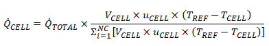
Heat Exchanger models are used to replicate the transfer of heat between two fluid streams - hot fluid and cold fluid. Applications include air conditioner evaporators, condensers, charge air coolers, radiators, electric heaters, and electronic devices. There are two options available:- Single stream option: in this case only one of the fluid streams (usually the cold stream) is modeled explicitly - by specifying the heat exchanger enthalpy source, while the second stream is assumed to have a uniform temperature that user specifies. This is activated by using option Heat Exchanger for Energy Source Option for the individual Region node.
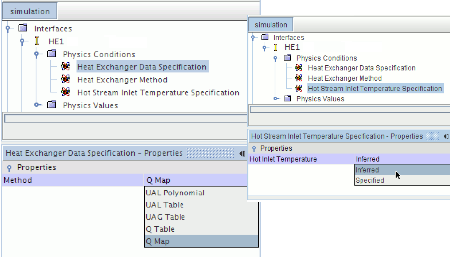
- Heat Exchanger Exit Temperature Specification is used to choose between specifying the heat transfer rate and predicting the outlet temperature or vice versa.
- Here V denotes volume of the cells, u the the velocity and NC refers to total number of cells. Note that there are 3 unknowns: local velocity, local temperature and local heat transfer rate.
- When this condition is chosen to be 'Inferred', the heat transfer rate can be specified by accessing the Heat Exchanger Energy Transfer physics value node.
- For a heater, the hot stream [e.g. coolant path in automotive radiator] is assumed to have an infinite thermal capacitance and the specified heat exchanger temperature TH refers to the constant temperature of the hot stream.
- For specified heat exchanger energy transfer rate Q, the inlet cold stream [e.g. air in automotive radiators] temperature TCI, and the cold stream specific heat CpC, an energy balance could be used to predict the cold stream exit temperature TCO as TCO = TCI + Q / CpC / mC where mC is mass flow rate of the cold fluid.
- Heat Exchanger First Iteration: This node specifies the iteration from which the heat exchanger enthalpy source is active and begins its contribution to the source term of the energy equation.
- It is recommended to active the source term when the flow is beginning to conform to its expected pattern, at least in terms of direction. As per user manual, 50 iterations is a good estimate to get a reasonable conformity.
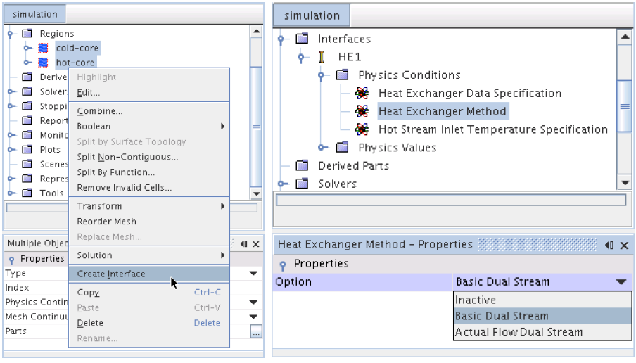
- Dual stream option: here both the streams are modeled explicitly by defining two overlapping regions and creating a heat exchanger interface between them. This model supports
- fluid-solid interface where the heat exchange occurs between a solid region and a fluid region and
- As seen in the expression, the heat transfer rate is calculate after dividing by average volume of the cells - it is recommended to keep the volume of the cells as uniform as possible.
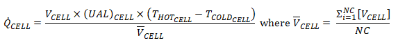
- fluid-fluid interface where the heat exchange takes place between two fluid regions. For a fluid-fluid type heat exchanger, following options are available for specifying heat transfer rate in the heat exchanger:
- UAL Polynomial [UAL is function of cold flow velocity], UAL Table [UAL is a table of the cold flow velocity], UAL Map [map of curves to specify the UAL directly when multiple heat exchanger curves]: UA refers to the product of the Overall heat transfer coefficient (U) and the Area of the heat exchanger (A). UAL refers to the local (or cell value of) heat transfer coefficient (in W/K), with L referring to local.
- UAG [U.A Global] Table
- Q Table [table of the cold stream mass flow rate for one value of hot stream mass flow rate], Q Map [series of curves from which it calculates UAL].
- Basic option: This option solves for a simpler version of the energy equation using only the convective term and the source term to yield a solution. Heat Exchanger Topology:
- When using the basic option, ensure that the core mesh is constructed of uniform cells.
- In other words, all the cells in the heat exchanger region must be of comparable cell volume, as the cell volumes do not enter the calculation of the UAL table in the basic model.
- The accuracy of results that the actual dual stream heat exchanger predicts does not depend on the uniformity of the mesh.
- The topology must contain two identical regions with a different continuum associated with each region.
- Both the regions [hot and cold streams] should be created from the same mesh continuum. To ensure this, copy the [core region of the radiator] region after the volume mesh has been generated.
- Once the two overlapping regions exist, the heat exchanger interface can then be created by selecting the two regions and choosing Create Interface from the right-click menu. While selecting the two regions, select the region representing the cold stream before the region representing the hot stream.
- The mesh alignment option should be activated so that a conformal match is obtained across mesh interfaces. STAR-CCM+ does not automatically generate a conformal mesh across interfaces for the trimmed cell mesh type. Operations > Automated Mesh > Meshers > Trimmed Cell Mesher node and activate Perform Mesh Alignment.
- Create a block shape part around the core which required for the volumetric controls that define mesh refinement. Geometry > Parts node and select New Shape Part > Block.
- Actual option: UAL Map method is available with the actual dual stream heat exchanger option only.
- In both the options, heat is added or removed from the core cells as a source or sink term in the corresponding fluid energy equation. It is assumed in this section that both the streams exist only in a single phase (liquid or gas) and no phase change occurs inside the heat exchangers.
Create Summary Report: STAR-CCM+ save a detailed report of simulation set-up in an HTML file. Use the feature File > Summary Report > To File... This file contains 35 top-level sections starting with | followed by characters +-1, +-2, ... , +-35 and three columns in a table. They are +-1 Continua, +-2 Interfaces, +-3 Regions, +-4 Representations, +-5 Automation, +-6 Contacts, +-7 Parts, +-8 3D-CAD Models, +-9 Operations, +-10 Descriptions, +-11 Coordinate Systems, +-12 Parametrizations, +-13 Tables, +-14 Units, +-15 Custom Trees, +-16 Voume Shapes, +-17 Idealizations, +-18 Color Palettes, +-19 Data Set Functions, +-20 User Code, +-21 Data Focus, +-22 Layouts, +-23 Data Mappers, +-24 Motions, +-25 Reference Frames, +-26 Screenplays +-27 Derived Parts, +-28 Summaries, +-29 Monitors, +-30 Reports, +-31 Solvers, +-32 Stopping Criteria, +-33 Solution Histories, +-34 Solution Views and +-35 Layout Views.
Second level options are created by adding additional | and last entry starts with `- instead of +-.|+- Regions ||+-1 Models ||+-2 Reference Values ||`-3 Initial ConditionsThe entry for Continua section is:
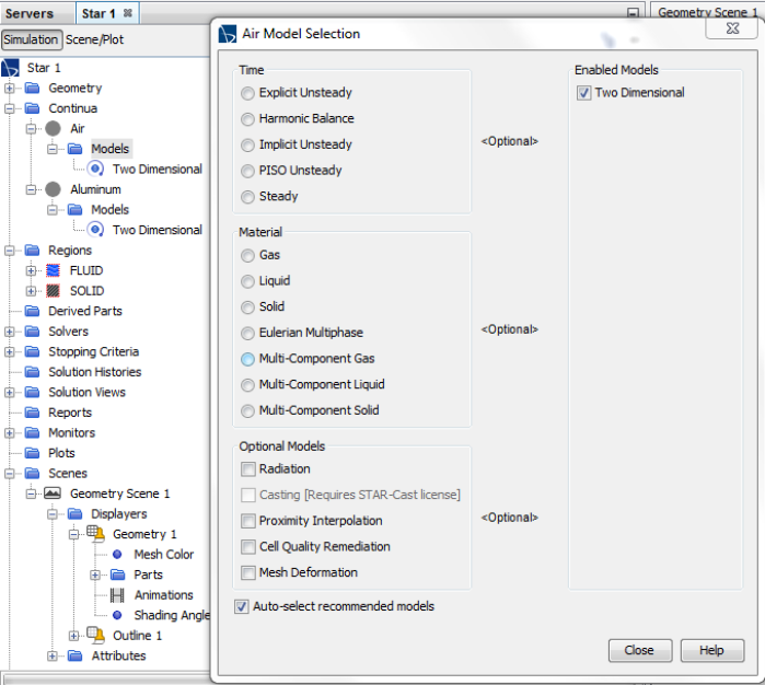
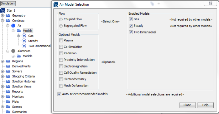
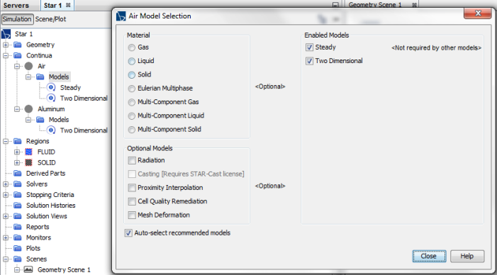
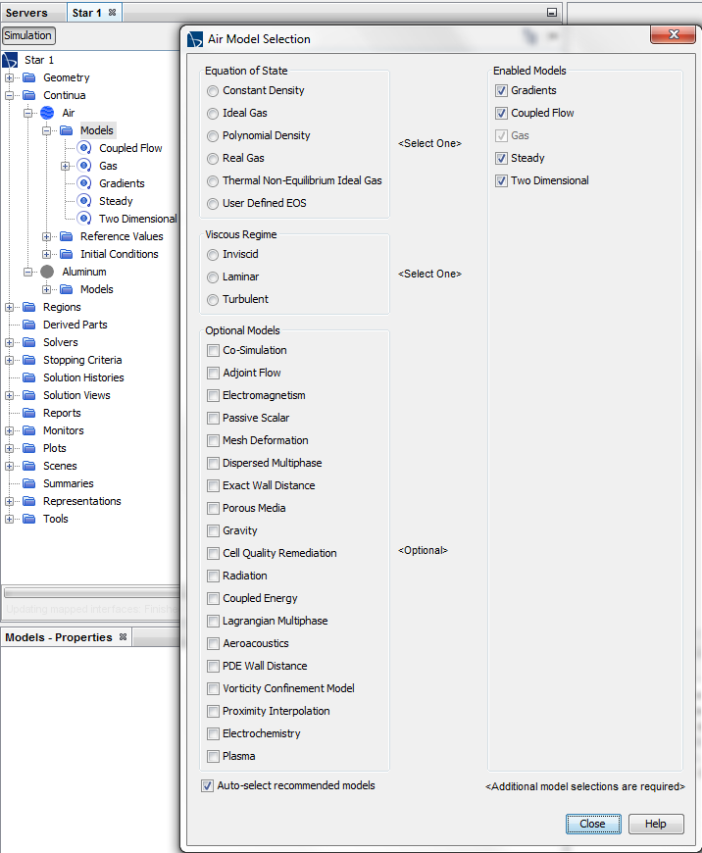
|+-1 Continua
||+-1 Air
|||+-1 Models
||||+-1 Cell Quality Remediation
||||+-2 Gas
||||+-3 Gradients
||||+-4 Gravity
||||+-5 Gray Thermal Radiation
||||+-6 Ideal Gas
||||`-7 Implicit Unsteady
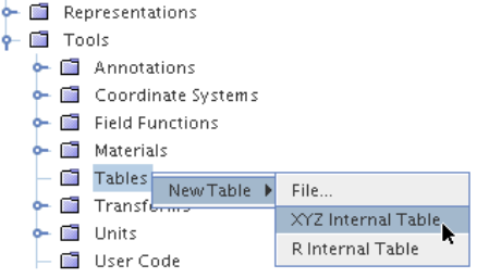
Initialize Solutions
It is easy to initialize a solution from previous runs if only boundary conditions are changed. In case where mesh is changed, the desired field variables (such as pressure, velocity and turbulence) should be extracted for each and every cell of old simulation using a table, XYZ Internal Table to be precise. Scalars selection field is used to open the scalars selection dialog box inside the table properties tab. To import the old values to new simulation file: expand 'Continua' object under model tree and navigate down to "Initial Conditions" tab. Choose Table (x,y,z) as option such as Pressure > Properties > Method > Table (x,y,z). Under Table (x,y,z) - Properties window, use drop-down available for Table: Data row, e.g. select 'Pressure' to initialize pressure field.Solution
STAR-CCM+ Lite can be used to post-process the results of simulations that were solved using STAR-CCM+ (ccmpsuite). STAR-CCM+ Lite can be used to run the simulation for further iterations providing all models are available in STAR-CCM+ Lite including Java macros that were generated by STAR-CCM+ (ccmpsuite). However, if the macro activates any models that are not permitted under the STAR-CCM+ Lite license, the simulation shall fail to run.
The stopping criteria in STAR is not incremental. That means, if stopping criteria is set to 4000 iterations and that many iterations are already completed, this value needs to be increased to 5000 when you modify (such as change inlet velocity) the *.SIM file and want to make additional 1000 iterations. In batch runs, the output of the program can be saved to a file: starccm+ -batch mySim.sim > log.text. For work in the interactive (GUI) client, check the option: Menu bar > Tools > Options > Environment > Log output to File.
As described in the user manual, Design Manager has two possible ways to submit: "General Job Submission" and "Pre-Allocation Job Submission". Single run (No Design Manager) - The single run submission is for cases where only a single simulation without the use of Design Manager is submitted. To submit to the cluster, the sim file and any macros are to be uploaded all in the same directory.
Batch Runs on HPC Clusters
The parallel batch (non-interactive or non-GUI) runs on local machines can be made using command line or from shell/batch files such as: [1]When batch or shell script and *.sim files are in same folder --- starccm+ -np 32 -batch javaFile.java simFile.sim [2]When batch or shell script and *.sim files are in different folders --- starccm+ -np 32 -batch javaFile.java folder1/sub-folder1/simFile.sim. starccm+ -batch geoImport.java, geoClean.java, geoReanme.java, mesh, step, run - multiple commands within the -batch argument can be specified, three macros are run in order before running the mesh pipeline, step and the solver.
If the properties in the simulation file are correctly set, many batch simulations can be run using the default operations with no java file: starccm+ -batch myCase.sim. For example, reports, auto-save, auto-export, and scene hardcopies can all be specified in the simulation properties. Command line to open the STAR-CCM+ workspace, start a new simulation, and play a macro: starccm+ -new -m macro.java Batch mode for macros is run from the command line using the -batch option: starccm+ -batch macro.java myCase.sim. This option runs STAR-CCM+ with a script (macro.java in the above example). The -batch option ensures that no GUI is displayed. If you do not want the server process to exit once the batch file has completed, then add the -noexit option to the command line.
Set File parameter from command line using -param command-line option. Change global parameter values without opening the GUI: Use the .ini input file to supply multiple parameter values at once.
The mesh generation in parallel is not scalable linearly, that is the speed-up is not proportional to the increase in number of cores (CPUs). Refer the image below from official documents: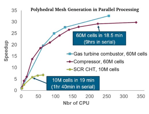
CHECKPOINT and ABORT: STAR-CCM+ runs can be aborted (saved at current iteration and exit the run) by creating a blank 'ABORT' file in home directory. A blank CHECKPOINT file shall save the simulation file at current iteration and let the run continue as per convergence setting.
Multiple Simulations Consecutively
Multiple simulation files can be loaded and run consecutively using a single macro. The following sample macro looks for all the .sim files in a specified directory, then for each simulation file it starts a server, iterates, and saves to a new filename. Use the command line: starccm+ -batch runMultiple.java. Save the macro as runMultipleCases.java and upload *.sim files along with this Java macro.
package macro;
import java.io.*;
import star.base.neo.*;
import star.common.*;
public class runMultipleCases extends StarMacro {

  // Create a file filter 'SimFileFilter' to list only *.sim files
  public class SimFileFilter implements FilenameFilter {
    //Test if a specified file should be included in a file list
    public boolean accept(File dir, String name) {
      return name.endsWith(".sim");
    }
  }

  public void execute() {
    // For runs on a cluster, folder path may not be known in advance
    // Change "." to local folder while running on a local host
    File simDir = new File(".");
    Simulation sim_0 = getActiveSimulation();

    sim_0.kill();
    for (File f : simDir.listFiles(new SimFileFilter())) {
      startAndRun(f);
    }
  }
  public void startAndRun(File f) {
    System.out.println("\n Starting "+f);
    String fileName = f.getAbsolutePath();
    Simulation sim_i = new Simulation(fileName);
    sim_i.getSolution().clearSolution();
    sim_i.getSimulationIterator().run();
    String nuName = fileName.replaceAll(".sim", "-new.sim");
    sim_i.saveState(nuName);
    sim_i.kill();
  }
}
Refer the tutorial "Solution Recording and Playback: Vortex Shedding" to know about recording solution histories, animating them and many other features of STAR. Node named "Simulation Operations" under Tools can be used to design a set of commands like meshing, running physics, setting different parameter value, clear solution, saving simulation, exporting scenes... though the options are applicable within the same simulation (*.sim) file.
Post-Processing
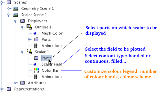
The plots in STAR are generated using scenes which are collection of 2 objects - Displayers and Outline. (a)Outline can be used to select section plane, boundary faces and edges (b)Scalar or vector - the actual component of contour plot - here again parts need to be selected on which contour plots are to be generated and (c)Attributes - this refers to features available to control the generation and display of the plots. In ANSYS Fluent as on V2021 R2, separate plots for mesh and scalar need to be generated. Then a scene needs to be manually created where required mesh plot and scalar plot can be combined which makes it close to the concept of Scenes used in STAR.
To animate streamlines: Click scene/plot > Edit the Displayers node > Streamline Stream 1 > Animations > Animation Mode > Tracers. Displayers > Streamline Settings > Delay between tracers (sec), Head size, Tail Length (sec)
Section Planes and Reports
The post-processing planes can be created under Derived Part tab in the Model Tree. Quantitative values such as area-averaged pressure needs to be defined under Reports tab in the Model Tree. The convergence history charts are available under tab Plots.Delete a report: While trying to delete a report from a sim file, following message shall appear: "<report name> is being used by another object and cannot be deleted". This means there are other objects in the simulation tree such as monitors and plots that are dependent on the report being removed. Clicking on the Details button shows the dependencies and gives the user the option to delete the report along with all the dependent objects, "Delete All" button.
Add Annotations: Expand the Tools > Annotations node and drag the appropriate node into the scene. Available built-in options are: Iteration, Logo, Scene, Solution Time, Time Step. The "Time Step" or "Solution Time" annotations are useful to track progress of transient simulations or creating animations to show time on each frame. Annotation gets added to the bottom left of the scene. One can add the annotation to a plot or a scene by drag-and-drop annotations from Tools > Annotations directly into scenes. Alternatively,for a scene, the annotations are found under Scene > Attributes > Annotations. Report annotations can be used to display values calculated by report on the graphical displayers in a scene.
Extra Post-processing
To check for zones or areas of very high gradients and residuals, turn on the Temporary Storage Retained option (accessed through solver properties panel). Running at least 1 iteration with this option gives access to additional field functions that can be used for troubleshooting poor convergences.License Manager: LMTOOLS
Most of the CFD programs be it ANSYS FLUENT or STAR-CCM+ use LMTools to manage the licenses at their customers. The executable utility is installed in the same folder where main program such as ANSYS FLUENT is installed. The syntax to use LMSTAT is: lmstat [-a] [-c license_file_list] [-f [feature]] [-i [feature]] [-s[server]] [-S [vendor]] [-t timeout_value]. The purpose of each option is:- -a: Displays all information
- -c license_files: Uses the specified license files
- -f [feature]: Displays 'users' of feature. If feature is not specified, all features are displayed
- -i [feature]: Displays information from the feature definition line for the specified feature, or all features if feature is not specified
- -s [server]: Displays status of all license files listed in $VENDOR_LICENSE_FILE or $LM_LICENSE_FILE on server, or on all servers if server is not specified
- -S [vendor]: Lists all users of vendor’s features
- -t timeout_value: Sets connection timeout to timeout_value which limits the amount of time 'lmstat' spends attempting to connect to server.
Finding Names of Feature: to use -f option, one need to know the exact names of feasures. This can be found in license.dat file or check the output from -a options. lmutil.exe lmstat -s licServers -f "feature_name"
For scripting and partial automation of pre-processing, solver and post-processing activities, refer to this section of scripting page.
For dealing with file handling in Linux and Windows, refer to short summary of shell scripting.
Java Macros
Batch mode for macros is run from the command line using the -batch option: % starccm+ -batch sim_1.java sim_1.sim. Playing Macros Within Macros: it is allowed to create a macro that calls other macros. Setting values using a macro follows the same logical sequence as expanding nodes in the object tree. Each of the entities in STAR-CCM+ is an object and to locate an object, the hierarchy of the object tree should be followed. For example, the initial velocity object is contained in a physics continuum object, which is contained in a simulation object.In JAVA, class name should always be the same as file name. If file contains multiple classes, only one class (or interface) in file can be public, and it must have the same name as file. it is not a requirement that "class name must always be the same as file name", the convention is to make one public and make sure that the file name matches. Other conventions: The prefix of a unique package name is always written in all-lowercase ASCII letters. Class names should be nouns, in mixed case with the first letter of each internal word capitalized. Interface names should be capitalized like class names. Methods should be verbs, in mixed case with the first letter lowercase, with the first letter of each internal word capitalized. To compile the file, "javac file_name.java", to run the generated class file, use file name without extension .java, that is "java file_name".
If classes are in separate files (e.g. main_class.java, class_1.java, class_2.java) and main_class.java is the one containing the main method and references other classes such as class_1.java, compiling main_class.java will also compile class*.java if the source files are present in the same directory. After successful compilation, the folder will have corresponding .class files for each Java file. To run the program, use the 'java' command followed by the name of the class that contains the public static void main(String[] args) method.To someone not familiar with OOP, there is steep learning curve further aggravated by concepts such as: Class Class<T>: T - the type of the class modeled by this Class object. For example, the type of String.class is Class<String>. Use Class<?> if the class being modeled is unknown. The terms like class, object, instance, type, interface, modifier... may get maddening initially. It is like asking someone to interpret: Name of man is man or Man is the name of Man.
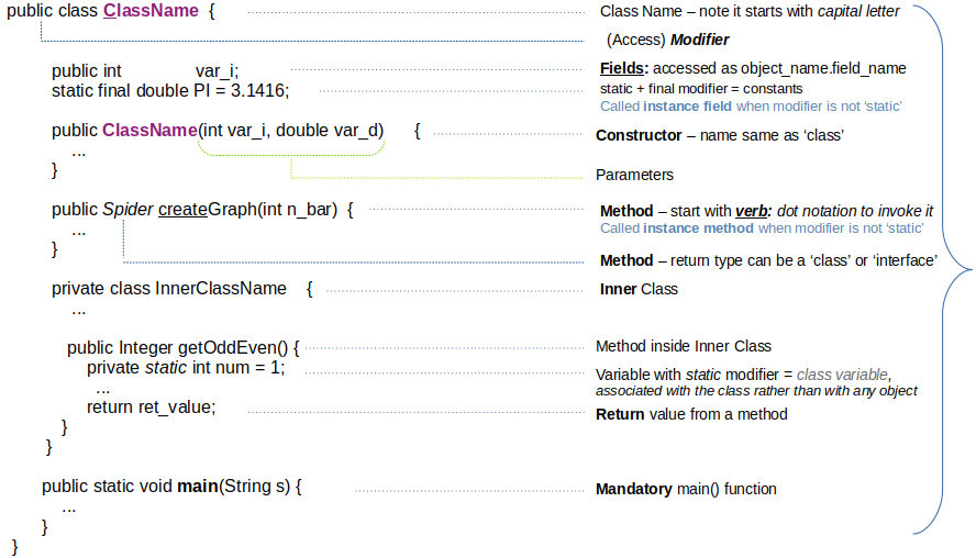
As per "docs.oracle.com/.../class/classNew.html" - chapter: "The .class Syntax" - A .class added to a class name references the class literal 'java.lang.classs', object that represents information about a given class. If the type is available but there is no instance then it is possible to obtain a Class by appending ".class" to the name of the type. Example: Class c = java.io.PrintStream.class; The variable 'c' will be the 'Class' corresponding to the 'type' java.io.PrintStream. If you think it is already complicated, refer two statements: "getClass() returns and instance (Object) of the Class class!" and "getClass() method returns the class of the object as a Class<T> object."
The user doc for Class Class<T> states: "Instances of the class Class represent classes and interfaces in a running Java application. Class has no public constructor. An enum class and a record class are kinds of class; an annotation interface is a kind of interface."
STAR-CCM+ Java API follows the naming convention mentioned in the image above. The .class is used when there is not an instance of the class variable where .getClass() is used there is an instance of the the class variable. obj_name.getClass() returns the 'class' of the 'object' obj_name.
- A 'class' provides blueprint for 'objects'
- An 'object' is created from a 'class'
- When an 'object' is created, an 'instance' of 'class' is created
- A 'class' contains 'constructors' that are invoked to create 'objects' from the class 'blueprint'
- As a convention, first letter of the name of a class should be capitalized (like a noun) - STAR-CCM+ API follows this
- "Instantiating a class" = "Creating an object"
- Child, sub, derived or inherited prefixes are used interchangeably as well as parent, super or base class
- To prevent other classes to inherit from a class, final keyword is used
- A 'class' can only extend one 'parent'
- Created 'object' is assigned to a 'variable'
- Simply declaring a reference variable does not create an object
- "TypeName reference_variable;" value will be undetermined until an object is actually created and assigned to it
- Member variables of a class are called 'fields'
- Variables accessible from all methods within a class are called instance variables or class variables (also known as static variables). They are declared inside the class, but outside any specific method, constructor, or block.
- Instance Variables (Non-Static Fields) belong to a specific object (instance) of a class. Each object created from the class has its own separate copy of the variable.
- Class variables (static variables) belong to the class itself, not any particular instance. There is only one single copy of the variable, shared by all objects of the class.
- Fields that have the static modifier in their declaration are called static fields or "class variables"
- Class variables are referenced by the class name itself: ClassName.ClassVar
- "Class variables" can be manipulated without creating an instance of the class
- All 'class' (should) have at least one 'constructor'
- 'Constructor' uses the same name as the 'class' and it has no 'return' value
- The name of 'constructor' provides the name of the 'class' to instantiate
- Except for 'Object' class, a 'class' has exactly one direct 'superclass'
- <U> Class<? extends U>: Casts this Class object to represent a subclass of the class represented by the specified class object.
- A 'method' can return 'primitive' or 'reference' type
- The declaration for a 'method' or a 'constructor' declares the number and the 'type' of the 'arguments' for that method or constructor
- A 'method' may use a 'class' name as 'return' type
- Variables in a method or block of code are called "local variables"
- As a convention, the first (or only) word in the name of a method should be a verb in lowercase - STAR-CCM+ API follows this
- An abstract method does not contain an implementation
- Static methods, which have the static modifier in their declarations, should be invoked with the class name, without the need for creating an instance of the class
- Derived or inherited class has access to all variables and methods of the parent class.
- The 'enum' declaration defines a 'class' (called an enum 'type') and enum class body can include 'methods' and other 'fields'
- An 'enum' type is a special data type that enables for a 'variable' to be a set of predefined 'constants'
- The members of an enum data type can have 'optional' value - refer enum data 'Day' below
- 'Parameters' refers to the list of 'variables' in a method declaration
- 'Arguments' are the actual 'values' that are passed in when the method is 'invoked'
- Defining an interface is similar to creating a new class
- Interfaces cannot be instantiated - they can only be implemented by classes or extended by other interfaces
- To use an interface, you write a class that implements the interface
- Classes can have fields, interfaces cannot
- When an instantiable class implements an interface, it provides a method body for each of the methods declared in the interface
- All constant values defined in an interface are implicitly public, static, and final and hence do not need to be explicitly defined - can be omitted
- Integer, Double, String, Boolean... are names of class and int, double, boolean... are types of primitive variable.
- Arrays have fixed size and stores primitives or objects, a List is an interface defining collection behavior, and an ArrayList is a dynamic, resizable class that implements the List interface.
- Arrays in Java
public class macroX extends StarMacro { ... }: A class called macroX is declared, and is specified as a subclass of the StarMacro class. public: informs the Java compiler that there are no access restrictions on this class, class: keyword to define a class, macroX: name of the class [must match the name of the file containing the class], extends: indicates that the class is derived from another class (and inherits all the public and protected methods of that class), StarMacro: name of the base class from which this one is derived.
Class StarMacro: public abstract class StarMacro extends RootMacro - Base class for all star macros. Re-implements Simulation methods to make final macros more concise and controlled. Constructor Summary: StarMacro() - Empty constructor. When you seach for a class in STAR-CCM+ Java API, the top content will be shown as described below for class SceneManager.Class SceneManager
java.lang.Object
star.base.neo.NeoJournalObject
...
star.common.GroupableSimulationObjectManager<Scene>
star.vis.SceneManager
Direct Known Subclasses:
...
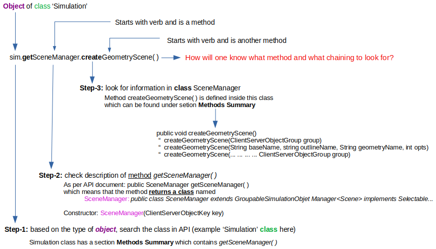
Method Chaining is a practice of using methods in a single line separated by dot (.) instead of calling methods with the same object reference separately. Each method in chaining returns an object and it discards the need for intermediate variables. Method chaining in Java is also known as "parameter idiom" or "train wreck" because of increased number of methods necessitating line breaks between methods. <> is known as "diamond operator".
Framework: a set of pre-defined classes, methods and interfaces which provide a ready-made set of tools to develop further applications. Like standard collection objects such as List<String> s_list = new ArrayList<String>() or Vector<Integer> v_idx = new Vector<Integer>(), STAR-CCM+ has objects pre-defined as per simulation objects such as Regions, Boundaries, Scenes... They can be defined as Collection<Region> regions = sim.getRegionManager.getRegions();
Summary of Java Programming relevant to STAR-CCM+ automation: case-sensitive, line terminated by semi-colon, // is single line comment, /* ... */ is multi-line comment
Member: variable belonging to a class, Method: subroutine belonging to a class, Instance Variable: variable contained in an object, Method Variable: subroutine contained in an object, Constructor: used to create new objects, dot operator is used to access field / variables / methods in a class object. Angle brackets, like html tags, containing one or more variables (separated by commas) refers to unspecified [declaring classes that use the generic type construct] type names: for example Collection<Part> allDerivedParts = pm_0.getObjects(); @Override annotation specifies the compiler that the method after this annotation overrides the method of the parent class: child method must have the same name and parameter(s) as in the parent class.
Languages like C, Java, and C++ require parenthesis '( ... )' around an entire expression when used in loops like if, while, or switch. A function need not be defined prior to accessing it so long the function and the calling statements are in same file. For each loop is shortened by using ':' such as "for (String strg : string_list)" is equivalent to "for each strg (which is of type String) in string_list". Double colon :: is called method reference operator.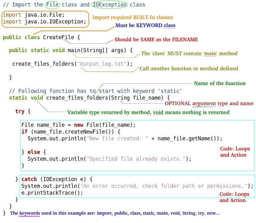
The demonstration Java file used above can be access here.
The @ symbol denotes a Java Annotation, attributes in C# which adds a special attribute to the variable, method, class, interface... the most common annotation is @Override, which indicates that a method is declared in a superclass. Similarly, @SuppressWarnings("unchecked") is another frequently used annotations.
More examples to refer simulation objects are given below. A 'collection' represents group of 'objects' known as its 'elements'. The Collection interface contains methods that perform basic operations, such as int size(), boolean isEmpty(), boolean contains(Object element), boolean add(E element), boolean remove(Object element), and Iterator<E> iterator().
Collection<Continuum> continuas = sim.getContinuumManager.getObjects();
Collection<Boundary> boundaries = sim.getBoundaryManager.getBoundaries();
Collection<Boundary> boundaries = sim.getBoundaryManager.getObjects();
Collection<Boundary> all_walls = new ArrayList<Boundary>;
Collection<Region> all_zones = new ArrayList<Region>;
Vector<Boundary> bound_list = Vector<Boundary>();
Collection<GeometryPart> geometry_parts = sim.getGeometryPartManager().getLeafParts();
Collection<Interface> interfaces = sim.getInterfaceManager().getObjects();
Collection<Tag> tag_list = massFlowReport.getTagGroup().getObjects();
Collection<PassiveScalarMaterial> passive_scalars = pc_1.getModelManager()
  .getModel(PassiveScalarModel.class)
  .getPassiveScalarManager().getPassiveScalarMaterials();
To loop on each type, one need to use the following construct:
for (object_type iterator_name : object_collection {
  ...
}
Here: object_type = GeometryPart or Region or Interface... and object_collection are the names all_walls or all_zones defined above.
Java API in STAR-CCM+
As per redhat.com: "APIs are sometimes thought of as contracts, with documentation that represents an agreement between parties: If party 1 sends a remote request structured a particular way, this is how party 2’s software will respond. APIs let you open up access to your resources while maintaining security and control. How you open access and to whom is up to you. API security is all about good API management, which includes the use of an API gateway. Opening technology to everyone, as with a public API, encourages developers to build an ecosystem of apps around your API. More people using your technology means more people are likely to do business with you."
Being a proprietary code, the API is not available in public domain and only a snippet can be produced if at all it can be. For example, the definition for the class FieldFunctionManager would be similar to described below. Here 'key' is the key of the server object. ClientServerObjectKey: Unique reference to an object on the server. ClientServerObject: Proxy base class for all objects that represent a server-side object.public class Simulation extends RootObjectRootObject: Server simulation proxy.
public class FieldFunctionManager
  extends FieldFunctionManagerBase
  implements ToolsManager
Manage Access to fieldFunction

Constructors:
  FieldFunctionManager(ClientServerObjectKey key)

Method Summary
Modifier and Type           Method                              Description
UserFieldFunction           createFieldFunction()                -
FieldFunction               getFunction(String functionName)     *
Collection<FieldFunction>   getScalarFieldFunction()             -
* Gets or creates the function with the given name. Similarly, the class FieldFunction is described in API as:
public abstract class FieldFunction
  extends FunctionProvider
  implements AbstractFunction...
STAR-CCM+ Java API contain section named as "Direct Known Subclasses". This is usually an extensive list of classes available. For example, Class ScalarProfile describes almost 250 direct known subclasses including ExternalEmissivityProfile, HeatFluxProfile, HeatSourceProfile, HeatTransferCoefficientProfile, ThermalResistanceProfile, ThermalContactResistanceProfile, TotalPressureProfile... These classes can be accessed as get(HeatSourceProfile.class).
Java API and as a matter of fact any API are similar to a dictionary: like any language, dictionary only serves as source of vocabulary and is useful if one is familiar with grammar, syntax or statement formation, morphology or word formation and semantics (how words, phrases, and sentences convey meaning). All these applies to any programming language and one can use API documents effectively only if they are familiar with it well.
API documents also get complicated as same method has different applications. Refer the example of getObject() below.
| Modifier | Type | Method | Description |
| Units | - | getObject(String name) | Look up object by toString() |
| <T extends ClientServerObject> | T | getObject() | Retrieve the ClientServerObject associated with this key |
Format and names of classes and methods in STAR-CCM+ are similar: for example get***Manager() where *** represents various components of simulation.
get|Continuum     |Manager(),  get|Region  |Manager()
get|Model         |Manager(),  get|Scene   |Manager()
get|PassiveScalar |Manager(),  get|Table   |Manager()
get|Representation|Manager(),  get|Report  |Manager()
get|Boundary      |Manager(),  get|Plot    |Manager()
and so on. The value of _x_ in classes named as get_x_Manager are: Annotation, CoordinateSystem, DataFocus, DataSet, Dfbi, Export, FeatureCurve, FieldFunction, GeometryPart, Groups, GlobalParameter, Layout, LicenseReservation, LookupTable, Mesh, Part, Monitor, PointSet, PartitionConfig, QueryFilter, ReferenceFrame, Report, Region, Presentation, SimulationSummary, Solver, SolverStoppingCriterion, Table, Transform, UpdateEvent, UserFunction, Units, View, VolumeShape
public void execute() {
  executeX();
}
The main method, execute(), is declared. When the macro is run in STAR-CCM+ it uses execute(), which calls executeX(). Instread of writing every line of code within execute(), other methods can be used as shown below:
public void execute() {
  genVolMesh();
  applyBC();
  makeRun();
}
void genVolMesh() {
  ...
}
void applyBC() {
  ...
}
void makeRun() {
  ...
}
import star.base.report.ScalarReport - here star.base.report is a package and ScalarReport is the class which has constructor ScalarReport(ClientServerObject key). Here, ClientServerObject is a class in package star.base.neo. STAR-CCM+ implements a client-server architecture where the GUI acts as the client and the simulation engine works as a server. Each object inside STAR-CCM+ simulation such as regions, boundaries and materials are represented by a CSO (ClientServerObject). To work with these objects, their CSO keys needs to be retrieved: for example, sim.MaterialProperty.GetObjects() returns a collection of all objects of type Collection<MaterialPropertyMethod> in the simulation.
Inheritance, like in dictionary meaning of heritage or act of inheriting property, refers to the concept of one object or class acquiring all the properties and behaviors of a parent object or class. It is a method to create new classes based on existing ones, reuse the methods and fields of parent class and if required add new fields and methods to newly created child class. The keyword 'extends' is used to implement inheritance in Java and can be applied to classes as well as interfaces. A new object is created as: objName instanceName = new objName(); note that objName is repeated, once without () and once with (). For example, Employees supervisors = new Employees(); Hashtable class provide key-value data structure like tuple and dictionaries in Python. Structure of inheritance is described below.
public class parentClass {

   public String field_x;
   public static void method_x() {
     ...
   }
   public static void method_y() {
     ...
   }
}
public class childClass extends parentClass {

  private int SIM_TYPE;
  private static void method_c() {
    ...
  }
}
class driverClass {

  childClass c_class = new childClass();
  System.out.println(c_class.method_x());
}
Interface is declared by keyword 'interface' and applied by keyword 'implements'. Java does not support "multiple inheritance" but a class can implement "multiple interfaces".
Private, Default, Protected, Public are called Access Modifiers in Java and control scope and access to a field, method, constructor, or class.
java.util.*: This Java package contains classes and interfaces designed to facilitate storing and manipulating groups of objects. This family of related interfaces and classes is called the Java collections framework.
When a wildcard is used in import statement, such as "import star.common.*", it does not include classes from subpackages. In other words, it imports classes directly only within the specified package. To include classes from a subpackage, they must be explicitly imported separately: for example "import star.common.graph.DataSet;". Ref: community.sw.siemens.com/s/.../macro-to-loop-through-internal-data-set-of-xy-plot
Some statements are put inside parentheses (...) and child classes are accessed with dots. The parentheses shown in bold fonts are optional and any space, tab, newline or combination of these characters are allowed before dot operators: PhysicsContinuum pc = ( (PhysicsContinuum) sim_1 .getContinuumManager() .getContinuum("Physics 1") ); In other words, any statement between a curly brace and semi-colon (;) or between semi-colon to next semi-colon are considered valid.
Try..Catch Loop: Almost all the programming languages have options for Exception Handling which are useful to handle cases when an error occurs, or 'exception' as it is referred as, the program or code stops and generates an error message. These exceptions are handled using the try ... catch statement in Java similar to try ... except block in Python.
try {
  ...codes...
} catch (IOException err) {
  sim_1.println("An error occurred while ...");
  err.printStackTrace();
}
A loop can be created over methods also: Runnable[] methods = {class_A:: method_A, class_B:: method_B, class_C:: method_C}; int i = 1; To run the require method: methods[i].run(); Normally the macro waits till the command is finished running. However, in case of complex problems requiring large memory and graphics power, the execution may jump to next statment before previous one is completed. This problem may occur with scenes where scene_x.initializeAndWait() can be used to circumvent this problem.
Built-in Methods in Java
Java built-in methods for strings note that keyword is 'String' to define this variable and int, float, char, boolean for other types: charAt(), codePointAt(), codePointBefore(), codePointCount(), compareTo(), compareToIgnoreCase(), concat(), contains(), contentEquals(), copyValueOf(), endsWith(), equals(), equalsIgnoreCase(), format(), getBytes(), getChars(), hashCode(), indexOf(), intern(), isEmpty(), join(), lastIndexOf(), length(), matches(), offsetByCodePoints(), regionMatches(), replace(), replaceAll(), replaceFirst(), split(), startsWith(), subSequence(), substring(), toCharArray(), toLowerCase(), toString(), toUpperCase(), trim(), valueOf()Java built-in methods for built-in arrays: compare(), copyOf(), deepEquals(), equals(), fill(), mismatch(), sort(). Property 'length' returns the length of an array.
Build-in methods for ArrayList, a resizable array: add(), addAll(), clear(), clone(), contains(), ensureCapacity(), forEach(), get(), indexOf(), isEmpty(), iterator(), lastIndexOf(), listIterator(), remove(), removeAll(), removeIf(), replaceAll(), retainAll(), set(), size(), sort(), spliterator(), subList(), toArray(), trimToSize().
Create an ArrayList object called 'employees' that will store strings: ArrayList<String> employees = new ArrayList<String>();
Java built-in methods for files: canRead(), canWrite(), createNewFile(), delete(), exists(), FileFilter(), FilenameFilter(), getAbsolutePath(), getName(), getParent(), getParentFile(), getPath(), isDirectory(), isFile(), length(), list(), listFiles(), mkdir()
How to use the macros described here? Common variables have been used in all the statements. Search for the variable such as zone name or boundary name for their definitions. The statements are listed as per simulation workflow though may not 100% comply with any specific sequence of GUI-based operations. Java macro in STAR-CCM+ can be used with standard Java functions and customized function for STAR. For example, getObject method, which is the most commonly used method for retrieving an object from within the repository, requires understanding of hierarchy in STAR-CCM+ repository. When using this method, one must fetch actual (Java) objects. To access attributes from that object, wrap the object in an invocation that calls the object’s getter methods. STAR-CCM+ Java API has getObjects() method which returns collection of objects. getModelManager() is used to get attributes of an object such as PhysicsContinuum.
Like API documents for Java programming itself such as "docs.oracle.com/javase/8/docs/api", STAR-CCM+ has its API available through Main Menu -> Help -> Java API. However, this document is not for beginners and does not contain any examples (they are not meant to serve purpose of textbooks or tutorials but acts more like an index or dictionary).The understanding of method to create an object in Java is critical to understand how macro can be developed for STAR-CCM+ such as: Creating object using 'new' keyword: className obj_name = new className(); Create object of Vector having type 'String': Vector<String> v_str = new Vector<String>(); where Vector is growable (resizable) array. This can be used to define a list of boundary and cell zones.
Creation of object in STAR: Units un_deg = (Units) sim_1.getUnitsManager() .getObject("deg"); Notice the similarity and difference between standard Java method and that followed in STAR-CCM+ macros. Note that the keyword new is not or rarely used in STAR-CCM+ which uses an Object Factory Pattern to create and manage objects within its simulation environment. The object creation is handled behind the scene which ensures that everything that needs to be there is in fact there. This approach makes it very difficult if not impossible to construct an instance of object that is unusable for any reason. When a macro is recorded, the GUI handles object creation behind the scene and hence the record macro feature does not need to explicitly use the 'new' keyword.
One extensively used concept is Collection in STAR-CCM+ which is not a pre-defined Object class but an interface for objects that store other objects. A familiarity with Factory, Factory Method and Abstract Factory is important to understand implementation of Java in STAR-CCM+ and published API.The methods starting with 'get' and 'set' are widely used in STAR. The get method returns the variable value, and the set method sets the value. These are used to access private variables which otherwise can only be accessed within the same class. Syntax for both is same: start with either get or set, followed by the name of the variable.
Summary of Java Syntax
Access elements of a list array by index: List<ObjectType> list_array = new ArrayList<ObjectType>(); ObjectType object_instance = list_array.get(n); int list_size = list_array.size();
physicsContinuum.getModelManager().has("Inviscid") is equivalent to following 3 lines of statement:Collection<Object> models = physicsContinuum.getModelManager().getChildren();
String model_names = models.toString();
Boolean is_inviscid = model_names.contains("Inviscid");
if (is_inviscid == true) {
...
}
- public Vector<Region> getRegions() - Return the collection of Regions assigned to this Continuum
- public Vector<Interface> getInterfaces() - Return the collection of Interfaces that reference Regions assigned to this Continuum
- public boolean hasRegion(Region region): Test whether the specified region is in this continuum.
- public static <T extends Continuum> T hasRegion(Region region, Class<T> clazz): Find the contuinuum of the specified class that contains the specified region
- public neoProperty getEnabledModels(): Returns the collection of enabld models in this continuum
- public Collection<Object> getChildren(): Get all objects
- sim.println(physicsContinnum.getModelManager().getChildren(): output may be [Three Dimension, Solution Interpolation, Gas, Segregated Flow, Gradients, Constant Density, Turbulent, Reynolds-Averaged Navier-Stokes, K-Epsilon Turbulence, Realizable K-Epsilon Two-layer, wall Distance, Two-layer All y+ Wall Treatment, Steady]
Get reference to active simulation: Simulation sim_1 = getActiveSimulation(); Print message in output log window: sim_1.println("\n Starting run for case " + "i");
Save simulation file:
sim_1.saveState(resolvePath( "./projects/newFileName.sim"));
sim_1.saveState(folder + "newFileName_" + i + ".sim");
sim_1.saveState("Y:\\CFD_Runs\\" + sim_1.getPresentationName() + "_new.sim");
Get name of the current sim file: String sim_file = sim_1.getPresentationName();
Close a session: When running in batch mode, the simulation will be closed automatically when end of macro is reached. For simulations via GUI: sim.close (ServerConnection.CloseOption. ForceClose);
Global Constants: Math.PI, Provided by java.lang.Math class can be used to access π e.g. deg2rad = angle * Math.PI/180; or use field functions:
UserFieldFunction uff_pi = sim_1.getFieldFunctionManager() .createFieldFunction();
uff_pi.setPresentationName("Pi");
uff_pi.setFunctionName("Pi");
uff_pi.setDefinition("3.1416");
Play a macro from within a macro: new StarScript(sim_1, new java.io .File(resolvePath( "createCsvReport.java" ))) .play();
Define Unit Vector: Units un_1 = sim_1.getUnitsManager( ).getPreferredUnits( new IntVecor( new int[] {...} ) ) which is equivalent to following lines of code.
Units un_len =
  sim_1.getUnitsManager().getPreferredUnits(
  new IntVector(
  new int[] {0, 1, 0, 0, 0, 0, 0, 0, 0, 0, 0, 0, 0, 0, 0, 0, 0}
  )
);
The 'UnitsManager' object through the call to 'getPreferredUnits' is used to find the 'Units' object that represents the default units in the active simulation. The value 0 or 1 are exponent to variables in the order Mass, Length, Time, Temperature, Current, Luminosity, Quantity, Angle, Temperature Difference, Solid Angle, Force, Energy, Power, Pressure, Velocity, Angular Velocity, Volume... getObject: starts with a verb and hence is a method. The getObject method is the most commonly used method for retrieving an object from within the repository.
Units un_mm = (Units) sim_1.getUnitsManager().getObject("mm"));
Units un_deg = (Units) sim_1.getUnitsManager().getObject("deg");
Units un_ang = sim_1.getUnitsManager() .getPreferredUnits( Dimensions .Builder() .angle(1).build());
Units un_len = sim_1.getUnitsManager() .getPreferredUnits( Dimensions .Builder() .length(1).build());
Units un_prs = (Units) sim_1.getUnitsManager() .getObject("Pa");
sim_1.getUnitsManager() .getSystemOption() .setSelected( UnitsManagerSystemOption .SYSTEM_USCS );
Units for density:
Units un_den = sim_1.getUnitsManager() .getPreferredUnits(new
  IntVector(new int[] {1, 0, 0, 0, 0, 0, 0, 0, 0, 0, 0, 0, 0, 0, 0, 0, -1, 0, 0, 0, 0, 0, 0, 0}));
Creating units using dimension builder:
HTC.setDimensions( Dimensions .Builder() .length(-2) .temperature(-1) .power(1) .build() );
Units un_celsius = (Units) sim_1.getUnitsManager() .getObject("C");
Create Dimensionless Unit: Applicable to variables like Pressure Coeffcients, Drag Coefficients... :
Units un_dim_less = sim_1.getUnitsManager() .getPreferredUnits(new IntVector(
  new int[] {0, 0, 0, 0, 0, 0, 0, 0, 0, 0, 0, 0, 0, 0, 0, 0, 0, 0, 0, 0, 0, 0, 0, 0, 0}) );
Pre-Processing
Create Import Manager: ImportManager im_1 = sim_1.getImportManager();
Import STL mesh: im_1.importStlSurface(resolvePath("D:\\Projects\\Geom.stl"), "OneBoundaryPerPatch", un_1, true, 1.0E-8);
Import a CAD Part:: PartImportManager p_im_mgr = sim_1.get(PartImportManager.class); p_im_mgr. importCadPart(reolvePath("D:\\Projects\\Geom.stp"), "SharpEdges", 30.0, 3, true, 1.0e-5, true, false, false, false, true, NeoProperty.fromString("{\'STEP\': 0, \'NX\': 0, \'CATIAVS\': 0, \'SE\': 0, \'JT\': 0}"), true, false);
Getting the name of the root directory or current working directory: String root_dir = sim_1.getSessionDir(); Get the right separator as per OS: String sep = System.getProperty("file.separator");
Create a folder and/or file:
Files.createDirectories( Paths.get(root_dir + "/field_data"));
File f_out = new File(resolvePath("Output.csv"));
FileReader f_reader = new FileReader(f_in);
BufferedReader b_reader = new BufferedReader(f_reader);
Scanner f_scan = new Scanner(b_reader) .useLocale(Locale.ENGLISH);
Define delimiter for .csv format: f_scan.useDelimiter(",");
Get name of a file: f_in.getName();
Delete a file: f_in.delete();
Check if a file exists: f_out.exists();
Define variables - all values are assumed to be in SI units: double holeDia; double TubeLength = 0.25; boolean isUnSteady = true; String TurbulenceModel = "RANS-kOmega"; int numPrismLayers = 10;
Select imported part for Mesh Generation: CadPart cadPart_1 = (CadPart) sim_1.get(SimulationPartManager.class) .getPart("Geom");
Apply mesh operation on a CAD part: AutoMeshOperation autoMeshCad = (AutoMeshOperation) sim_1.get(MeshOperationManager .class) .createAutoMeshOperation(new String [] {"star.resurfacer .ResurfacerAutoMesher"}), new NeoObjectVector( new Object[] {cadPart_1});
Do operations based on names:
String bnd_name = 'inlet';
for (Boundary bnd : boundaries) {

  if (bnd_name.equals(bnd.getPresentationName()) {
    ...
  }
}
for (PartSurface srf : part_surfaces) {

  if (bnd_name.equals(srf.getPresentationName()) {
    ...
  }
}
Define mesh sizes, apply Automesh operation and generate volume mesh: Here, Auto_Mesh is object defined under node 'Operations'.
autoMeshCad.getDefaultValues() .get(BaseSize.class) .setValue(0.1);
autoMeshCad.getDefaultValues .get(BaseSize.class) .setUnits(un_1);
AutoMeshOperation autoMesh = (AutoMeshOperation) sim_1.get(MeshOperationManager.class).getObject("Auto_Mesh");
autoMeshOperation .execute();
MeshPipelineController v_mesh = sim_1.get( MeshPipelineController.class );
v_mesh.generateVolumeMesh();
v_mesh.ClearGeneratedMeshes();
Check existence and create mesh continuum:
Collection<Object> continua = sim.getContinuumManager().getChildren();
for (Object obj : continua) {
  if (obj instanceOf MeshContinuum) {
    ...
  }
}
MeshContinuum meshCont = sim_1.getContinuumManager().createContinuum (MeshContinuum.class);
meshCont.enable(ResurfacerMeshingModel.class);
meshCont.getReferenceValues() .get(BaseSize.class) .setValue(2.0);
Translate Mesh: sim_1.getRepresentationManager() .translateMesh( new NeoObjectVector( new Object[] {zone_htx}), new DoubleVector( new double[] {0.0, del_y, 0.0} ), new NeoObjectVector( new Object[] {un_mm, un_mm, un_mm}), CartCS );
Rotate Mesh: sim_1.getRepresentationManager() .rotateMesh( new NeoObjectVector( new Object[] {zone_mrf}), new DoubleVector( new double[] {0.0, 0.0, 1.0}), new NeoObjectVector( new Object[] {un_mm, un_mm, un_mm}), rot_angle, CartCS);
At this stage, it is useful to have a macro which prints all the mesh operations and refinements that are present in the simulation. This could be the step to make statistics about mesh as a more automated process. One may try following lines to print sample information:
MeshContinuum meshContinuum = (MeshContinuum) sim_1.getContinuumManager().getContinuum("Mesh 1");
Collection<Object> mesh_obj = meshContinuum.getModelManager().getChildren();
String mesh_ops = mesh_obj.toString();
Check if the mesh contains polyhdral mesh
  public boolean isPoly(MeshContinuum mesh_continua){
    if(mesh_continua.getEnabledModels().containsKey("star.dualmesher.DualMesherModel")) {
      return true;
    } return false;
  }
Save mesh quality report in a text file and process using any other method such as VBA scripting.
FvRepresentation mesh_q_stats = (FvRepresentation) sim.getRepresetationManager().getObject("Volume Mesh");
Region r_fluid = sim_1.getRegionManager().getRegion("air_domain");
Region r_solid = sim_1.getRegionManager().getRegion("heat_sink");
mesh_q_stats.generateCompactMeshReport(new NeoObjectVector(new Object[] {r_fluid, r_solid}));
//Full Report
mesh_q_stats.generateMeshReport(new NeoObjectVector(new Object[] {r_fluid, r_solid}));
The text printed in output window can be stored in a String class and later saved into a text file:
String qSummary = mesh_q_stats.generateMeshReport(
  new NeoObjectVector(new Object[] {r_fluid, r_solid} ));
Define Boundary Conditions
Get a fluid region: Region zn_1 = sim_1.getRegionManager() .getRegion("air_domain");
public boolean hasRegion(Region region): test whether the specified region is in this continuum. public static <T extends Continuum> T hasRegion(Region region, Class<T> cls): find the continuum of the specified class that contain the specified region, returns null if the continuum does not exist.Get name of a zone: Boundary bnd_inlet = zn_1.getBoundaryManager() .getBoundary("inlet");
Demo of Upper Bounded Wildcards: upper bounded wildcard is used to relax the restrictions on a variable. Use the wildcard character '?' followed by the 'extends' keyword, followed by its upper bound. Here, 'extends' means either "extends" (as in classes) or "implements" (as in interfaces). The term List<Boundary> is more restrictive than List<? extends Boundary> because the former matches a list of type Boundary only, whereas the latter matches a list of type Boundary or any of its subclasses.
public Object lookupObject(Class<?> cls);                   <- as described in API
PhysicsContinuum pc = lookupObject(PhysicsContinuum.class); <- example statement
if (pc == null) {
  ...
}
private void createBoundary(Class <? extends BoundaryType> type) {
...
Boundary bnd = ....
bnd.setBoundaryType(type);
}
createBoundary(InletBoundary.class);
createBoundary(OutletBoundary.class);
createBoundary(WallBoundary.class);
Change the name of a continuum from "Physics 1" to 'air_domain': PhysicsContinuum pc_1 = (PhysicsContinuum) sim_1.getContinuumManager() .getContinuum("Physics 1"); pc_1.setPresentationName("air_domain"); To delete a continuum: sim_1.deleteObjects(new NeoObjectVector(new Object[] {air_domain})); Add a region to a continuum: air_domain.add(zn_1);
Contextual Focus to expand the physics model manager node and collapse other nodes: selectAndExpandNodeExclusive( pc_1.getModelManager() ); To exapand a node without affecting other open nodes, use selectAndExpandNode. To expand material property node: selectAndExpandNode( gas_0.getMaterialProperties() .getMaterialProperty( DynamicViscosityProperty .class ) .getMethod());
Set Coupled Solver:
CoupledFlowModel coupledFlow = pc_1.getModelManager() .getModel(CoupledFlowModel.class);
coupledFlow.getCoupledInviscidFluxOption() .setSelected(CoupledInviscidFluxOption.ROE_SCHEME);
Enable Solvers:
pc_1.enable(SteadyModel.class);
pc_1.enable(SingleComponentGasModel.class);
pc_1.enable(IdealGasModel.class);

SegregatedFlowModel seg_flow_mod = pc_1.getModelManager()
  .getModel(SegregatedFlowModel.class);
seg_flow_mod.getUpwindOption().setSelected(FlowUpwindOption.FIRST_ORDER);
SegregatedFluidTemperatureModel seg_fluid_tp = pc_1.getModelManager()
  .getModel(SegregatedFluidTemperatureModel.class);
seg_fluid_tp.getUpwindOption().setSelected(UpwindOption.FIRST_ORDER);

pc_1.enable(CoupledFlowModel.class);
pc_1.enable(CoupledEnergyModel.class);
pc_1.enable(TurbulentModel.class);
pc_1.enable(RansTurbulenceModel.class);
pc_1.enable(KEpsilonTurbulence.class);
pc_1.enable(RkeTurbModel.class);
RkeTurbModel rkeTurbMod = pc_1.getModelManager().getModel(RkeTurbModel.class);
rkeTurbMod.getUpwindOption().setSelected(UpwindOption.FIRST_ORDER);
pc_1.enable(KeHighYplusWallTreatment.class);
pc_1.enable(KOmegaTurbulence.class);
pc_1.enable(SstKwTurbModel.class);
pc_1.enable( KwAllYplusWallTreatment.class);
Check for available continua:
for (Continuum c : getsimulation().getContinuumManager().getObjects()) {
  if(c.getModelManager().hasModel(RadiationModel.class) != null) {
    ...
  }
  if(c. getModelManager().hasModel(SteadyModel.class) != null) {
    ...
  }
}
Turn ON Radiation:
pc_1.enable(GrayThermalRadiationModel .class);
GrayThermalRadiationModel gray_radiation = pc_1.getModelManager() .getModel(GrayThermalRadiationModel.class);
RadiationTemperature T_rad = gray_radiation.getThermalEnvironmentManager() .get(RadiationTemperature.class);
T_rad.getEnvRadTemp() .setValue(500.0);
Check type of domain or region:
public enum PhysicsRegionType extends Enum<PhysicsRegionType> where "Enum Class PhysicsRegionType" are: GAS_REGION, GAS_REGION2, LIQUID _REGION, MULTIPLE_TYPES, NETWORK_REGION, POROUS_REGION, SOLID_REGION, VOID_REGION
public class x_Region extends RegionType: Get fluid region type: x_ = Fluid, Solid, Porous
Define Material Properties - Density:
pc_1.enable(ConstantDensityModel .class);
SingleComponentGasModel single_gas_model = pc_1.getModelManager() .getModel(SingleComponentGasModel .class);
Gas gas_0 = (Gas) single_gas_model.getMaterial();
ConstantMaterialPropertyMethod constant_density = (ConstantMaterialPropertyMethod)
  gas_0.getMaterialProperties() .getMaterialProperty(ConstantDensityProperty.class).getMethod();
constant_density.getQuantity().setValue(1.225);
Define Polynomial Density for a Liquid:
SingleComponentLiquidModel liq_density = pc_1.getModelManager() .getModel(SingleComponentLiquidModel.class);
Liquid water = (Liquid) liq_density.getMaterial();
TemperaturePolynmial poly_density = (TemperaturePolynmial)
  water.getMaterialProperties() .getMaterialProperty( PolynomialDensityProperty .class) .getMethod();
Define Incompressible Ideal Gas and Constant Value or Sutherland Model for Viscosity:
IdealGasModel idealGas = pc_1.getModelManager() .getModel(IdealGasModel .class);
idealGas.setIncompressible(true);
SingleComponentGasModel gas_model = pc_1.getModelManager() .get_model(SingleComponentGasModel .class);
Gas gas_0 = (Gas) gas_model.getMaterial();
gas_0.getMaterialProperties() .getMaterialProperty(DynamicViscosityProperty.class) .setMethod(SutherlandLaw .class);
ConstantMaterialPropertyMethod visc = ConstantMaterialPropertyMethod
  gas_0.getMaterialProperties(DynamicViscosityProperty.class) .getMethod();
visc.getQuantity().setValue(1.716e-5);
SolidComponent solid_cs = (SolidComponent)
  getMaterials().getComponents().getComponent("heat_sink");
ConstantMaterialPropertyMethod rho_s = (ConstantMaterialPropertyMethod)
  solid_cs.getMaterialProperties().getMaterialProperty(ConstantDensityProperty.class).getMethod();
rho_s.getQuantity().setValue(rho_cs.doubleValue());
ConstantSpecificHeat cp = (ConstantSpecificHeat)
  solid_cs.getMaterialProperties().getMaterialProperty(SpecificHeat Property.class).getMethod();
cp.getQuantity().setValue(cp_cs.doubleValue());
Define polynomical Specific Heat and Thermal Conductivity. public DoubleVector(Collection<?> v): Constructs a vector containing the elements of the specified collection, in the order they are returned by the collection's iterator. Presumes the elements of the collection are Numbers, and converts them to Double if needed. void setCoefficients (DoubleVector v) and public void setExponents (DoubleVector v) are the methods required.
PhysicsContinuum pc = (PhysicsContinuum) sim.getContinuumManager().getContinuum("Steel");
SolidModel steel = pc.getModelManager).getModel(SolidModel.class);
Solid s_steel = (Solid) steel.getMaterial();

s_steel.getMaterialProperties().getMaterialProperty(SpecificHeatProperty.class)
  .setMethod(PolynomialSpecificHeat.class);
PolynomialSpecificHeat Cp_Poly_T = (PolynomialSpecificHeat) s_steel.getMaterialProperties()
  .getMaterialProperty (SpecificHeatProperty.class).getMethod();
Polynomial poly_cp = Cp_Poly_T.getPolynomial();
poly_cp.setNumberOfCoefficients(new IntVector(new int[] {4})) ;
poly_cp.setCoefficients(new DoubleVector(new double [] {0.1, 0.2, 0.3, 0.4)));
poly_cp.setExponents(new DoubleVector(new double[] (0.0, 1.0, 2.0, 3.0}));
poly_cp.setUseRealExponents(false);

s_steel.getMaterialProperties().getMaterialProperty(ThermalConductivityProperty.class)
  .setMethod(TemperaturePolynomial.class) ;
TemperaturePolynomial k_Poly_T = (TemperaturePolynomial) s_steel.getMaterialProperties()
  .getMaterialProperty(ThermalConductivityProperty.class).getMethod();
Polynomial poly_k = k_Poly_T.getPolynomial();
poly_k.setNumberOfCoefficients (new IntVector (new int[] {2}));
poly_k.setCoefficients(new DoubleVector(new double [) {0.02, 0.01}));
poly_k. setExponents(new DoubleVector(new double[] {0.0, 1.0}));

s_steel.getMaterialProperties().getMaterialProperty(ThermalConductivityProperty.class)
  .setMethod (OrthotropicThermalConductivityMethod.class);
OrthotropicThermalConductivityMethod ortho k = (OrthotropicThermalConductivityMethod)
  s_steel.getMaterialProperties().getMaterialProperty(ThermalConductivityProperty.class).getMethod();
Units un_k = (Units) sim.getUnitsManager().getObject("W/m-K");
ConstantMaterialPropertyMethod k11 = (ConstantMaterialPropertyMethod)
  (ScalarMaterialCoefficient) ortho_k.getScalarProperty(0).getMethod();
k11.getQuantity().setValueAndUnits(1.0, un_k);
ConstantMaterialPropertyMethod k22 = (ConstantMaterialPropertyMethod)
  (ScalarMaterialCoefficient) ortho_k.getScalarProperty(1).getMethod();
k22.getQuantity().setValueAndUnits(2.5, un_k);
ConstantMaterial PropertyMethod k33 = (ConstantMaterialPropertyMethod)
  (ScalarMaterialCoefficient) ortho_k.getscalarProperty(2).getMethod();
k33.getQuantity().setValueAndUnits (5.0, un_k);
Define Reference Pressure:
Units un_pr_atm = (Units) sim_1.getUnitsManager() .getObject( "atm" );
pc_1.getReferenceValues() .get(ReferencePressure .class) .setUnits(un_pr_atm);
pc_1.getReferenceValues() .get(ReferencePressure .class) .setValue(1.0);
Print all regions and number of boundaries:
for (Region r : getActiveSimulation().getRegionManager().getRegions()) {
  r_name = r.getPresentationName()
  System.out.println(r_name + ", " + r.getBoundaryManager() .getBoundaries().size());
}
Change name of boundary: bz_i.setPresentationName("mf_inlet");
VelocityProfile vp_1 = bz_i.getValues() .get(VelocityProfile.class); vp_1.getMethod( ConstantVectorProfileMethod .class) .getQuantity() .setComponents(10, 0, 0);
Mass Flow Profile at Inlet:
Boundary bnd_inlet = zn_1.getBoundaryManager().getBoundary(b_inlet);
MassFlowRateProfile mf_p = bnd_inlet.getValues().get(MassFlowRateProfile.class);
mf_p.getMethod(ConstantScalarProfileMethod.class).getQuantity() .setValue( 0.5 );
Use StaticPressureProfile.class and Constant ScalarProfileMethod.class to get and set pressure boundary conditions.
public void setInletBoundaries(Simulation simX, Region fluid_zone,
  Boundary b_inlet, double inlet_pr, double b_inlet_ti, double b_inlet_dh) {

  //Set boundary conditions of type "Total Pressure" on inlet(s). This function
  //can be used for outlets: change b_inlet to b_outlet.
  Boundary bnd_inlet = fluid_zone.getBoundaryManager().getBoundary(b_inlet);

  bnd_inlet.setBoundaryType(StagnationBoundary.class);
  bnd_inlet.getConditions().get(KeTurbSpecOption.class)
    .setSelected(KeTurbSpecOption.Type.INTENSITY_LENGTH_SCALE);
  // Options: INTENSITY_VISCOSITY_RATIO, K_EPSILON, K_OMEGA
  TotalPressureProfile tot_pr_in = bnd_inlet.getValues().get(TotalPressureProfile.class);
  tot_pr_in.getMethod(ConstantScalarProfileMethod.class).getQuantity().setValue(inlet_pr);

  TurbulenceIntensityProfile ti_in = bnd_inlet.getValues().get(TurbulenceIntensityProfile.class);
  ti_in.getMethod(ConstantScalarProfileMethod.class).getQuantity().setValue(b_inlet_ti);
  TurbulentLengthScaleProfile tl_in = bnd_inlet.getValues().get(TurbulentLengthScaleProfile.class);
  tl_in.getMethod(ConstantScalarProfileMethod.class).getQuantity().setValue(b_inlet_dh);
}
public boolean evaluate (Region region) {
Collection<Boundary> boundaries = sim.region.getBoundaryManager().getBoundaries()
for (Boundary bnd : boundaries) {
  BoundaryType boundaryType = bnd.getBoundaryType();
  if (boundaryType != null) {
    Class<? extends BoundaryType> boundaryTypeClass = boundaryType.getClass();
    if (boundaryTypeClass.equals(WallBoundary.class)) {
       w++;
    } else if (boundaryTypeClass.equals(PressureBoundary.class)) {
       p++;
    } else if (boundaryTypeClass.equals(InletBoundary.class)) {
      i++;
    }
  }
  VelocityMagnitudeProfile vMagProfile = boundary.getValues().has(VelocityMagnitudeProfile.class);
  if (vMagProfile == null) {
     ...
  }
  ProfileMethod vMagProfileMethod = VMagProfile.getMethod();
  if (!(vMagProfileMethod instanceof ConstantScalarProfileMethod)) {
     ...
  }
  Boundary boundary = region.getBoundaryManager().getBoundary(name_bound[i]);
  if (boundary.getValues().has(StaticPressureProfile. class) == null) {
    ...
  }
  if (boundary.getValues().has (VelocityMagnitudeProfile.class) == null) {
    ...
  }
}
Get interface boundary, convert wall to interface and change interface type:
BoundaryInterface b_iface = (BoundaryInterface) sim_1.getInterfaceManager() .getInterface("fin_air");
InternalInterface int_face = (InternalInterface) sim_1.get( ConditionTypeManager.class )
  .get( InternalInterface.class );
b_iface.setInterfaceType(int_face);
BaffleInterface baf_iface = (BaffleInterface) sim.get( ConditionTypeManager.class )
  .get( BaffleInterface.class );
b_iface .setInterfaceType(baf_iface);
Check if a boundary is solid-fluid interface
  public boolean isFluid(Boundary bnd){
    //Does this Boundary belongs to Fluid Region?
    return isFluid(bnd.getRegion());
  }
  public boolean isFluid(Region region){
    //Is this a Fluid Region?
    if(region.getRegionType().toString().equals("Fluid Region")) return true;
    return false;
  }
  public boolean isFluidSolidInterface(Interface iface_pair){
    Region reg0 = iface_pair.getRegion0();
    Region reg1 = iface_pair.getRegion1();
    if(isFluid(reg0) && isSolid(reg1)) return true;
    if(isFluid(reg1) && isSolid(reg0)) return true;
    return false;
  }
Specify Symmetry Boundary:
Boundary b_sym = zn_1.getBoundaryManager() .getBoundary("Symmetry");
b_sym.setBoundaryType( SymmetryBoundary.class );
Specify wall boundary conditions
AmbientTemperatureProfile Tref = boundary.getValues().get(AmbientTemperatureProfile.class);
Units units = (Units) simulation.getUnitsManager().getobject("C");
HeatTransferCoefficientProfile htc = boundary.getValues().get(HeatTransferCoefficientProfile.class);
units = ((Units) sim.getUnitsManager().getobject ("W/m^2-K"));
(ConstantScalarProfileMethod) htc.getMethod().getQuantity().setUnits(units);
(ConstantScalarProfileMethod) htc.getMethod().getQuantity().setValue (bound_htc);

if (boundary.getValues().has("Heat Flux")) {
  HeatFluxProfile heat_flux = (HeatFluxProfile) boundary .getValues().get (HeatFluxProfile.class) ;
Units units = (Units) sim.getUnitsManager().getObject("W/m^2");
(ConstantScalarProfileMethod) heat_flux.getMethod().getQuantity().setUnits(units);
(ConstantScalarProfileMethod) heat_flux.getMethod().getQuantity().setValue(bound_flux);
}
if (boundary.getValues().has("Static Temperature")) {
  StaticTemperatureProfile static_t = boundary.getValues().get(StaticTemperatureProfile.class) ;
  Units units = (Units) sim.getUnitSManager).getobject("C");
  (ConstantScalarProfileMethod) static_t.getMethod().getQuantity().setUnits(units);
  (ConstantScalarProfileMethod) static_t.getMethod().getQuantity().setValue(bound_temp);
}
Specify Heat Sources: zone_hs is variable holding name of the zone containing heat-source.
Region region_hs = sim_1.getRegionManager() .getRegion(zone_hs);
HeatSourceProfile hsrc = region_hs.getValues().get(HeatSourceProfile.class);
Units un_kW = (Units) sim_1.getUnitsManager().getobject("kW");
hsrc.getMethod(ConstantScalarProfileMethod .class) .getQuantity() .setUnits(un_kW);
hsrc.getMethod(ConstantScalarProfileMethod .class) .getQuantity() .setValue(0.10);
Create Parameters: these parameters can be used as design variables.
ScalarGlobalParameter scGlobalPar = (ScalarGlobalParameter)
  sim_1.get(GlobalParameterManager.class)
  .createGlobalparameter(ScalarGlobalParameter.class, "Scalar");
Units un_len = (Units) sim_1.getUnitsManger().getObjects("m");
scGlobalPar.getQuantity().setValueAndUnits(2.0, un_len);
scGlobalPar.setDimensions(Dimensions.Builder().length(1).time(-1).build());
Create Cartesian Coordinate System:
LabCoordinateSystem labCS_cart = sim_1.getCoordinateSystemManager( ) .getLabCoordinateSystem( );
CartesianCoordinateSystem CartCS = labCS_cart.getLocalCoordinateSystemManager()
  .createLocalCoordinateSystem( CartesianCoordinateSystem .class, "Cartesian");
Coordinate originCS = CartCS.getOrigin();
Units un_cs = (Units) sim_1.getUnitsManager() .getObject("m");
originCS.setCoordinate(un_cs, un_cs, un_cs, new DoubleVector(new double[] {0.1, 0.2, 0.0}));
Create Cylindrical Coordinate System:
LabCoordinateSystem labCS_cyl = sim_1 .getCoordinateSystemManager()
  .getLabCoordinateSystem();
CylindricalCoordinateSystem CCS = labCS_cyl .getLocalCoordinateSystemManager()
  .createLocalCoordinateSystem( CylindricalCoordinateSystem .class, "Cylindrical" );
CCS.setBasis0( new DoubleVector( new double[] {0.0, 1.0, 0.0}) );
Set Gradient Model:
GradientsModel gradModel = pc_1.getModelManager().getModel(GradientsModel.class);
gradModel.getGradientMethodOption() .setSelected(GradientMethodOption.GAUSS_GRADIENTS);
Set Translational and Rotation Motion, Rotating and Translating Reference Frame:
TranslatingMotion v_x = sim_1.get(MotionManager.class) .createMotion(TranslatingMotion .class, "Translation");
Units un_v_x = sim_1.getUnitsManager() .getInternalUnits( new IntVector(new int[]
  {0, 0, 0, 0, 0, 0, 0, 0, 0, 0, 0, 0, 0, 0, 1, 0, 0, 0, 0, 0, 0, 0, 0, 0}));
v_x.getTranslationVelocity() .setDefinition("$$x_v");
UserRotatingAndTranslatingReferenceFrame rot_trans_ref_frame =
  (UserRotatingAndTranslatingReferenceFrame)
  sim_1.get( ReferenceFrameManager .class) .getObject("Rotating And Translating");
rot_trans_ref_frame.getTranslationVelocity().setComponents(0.0, v_trans_y, 0.0);
MotionSpecification motion_zone = zone_mrf.getValues() .get( MotionSpecification.class );
motion_zone.setReferenceFrame( rot_trans_ref_frame );
RotatingMotion rot_X = (RotatingMotion) sim_1.get(MotionManager.class) .getObject("Rotation");
SuperposingRotatingMotion rot_Y = (SuperposingRotatingMotion)
  rot_X.getSuperposingMotionManager() .getObject( "Pitch" );
Create Field Monitor:
FieldMeanMonitor FMM = sim_1.getMonitorManager() .createMonitor(FieldMeanMonitor.class);
FMM.getParts().setQuery(null);
FMM.getParts().setObjects(zn_1);
FMM.setFieldFunction("FF_name";
FMM.setPresentationName("Monitor Name");
Set S2S radiation parameters and Calculate View Factorfor S2S Radiation Model. Radiation view factor summary printed in output window stored in variable vfSummary:
PatchPerBFaceProportion n_patch_face =  zn_1.getValues(getPatchPerBFaceProportion .class);
PatchPerBFaceLeaf n_patch_per_leaf = n_patch_face.getModelPartValue();
n_patch_per_leaf.setValue(20.0);
SharpAngle sharp_angle = zn_1.getValues() .get(SharpAngle .class);
sharp_angle.setSharpAngle(175.0);
ViewfactorCalculationSolver VFcalc = (ViewfactorCalculatorSolver)
  sim_1.getSolverMananger() .getSolver(ViewfactorCalculation.class);
VFcalc.generatePatches();
VFcalc.calculateViewfactors();
VFcalc.displayViewfactorSummary();
String vfSummary = VFcalc.getViewfactorSummary();
Define Porous Boudary Conditions: Set the inertial and viscous resistance in X-direction. Resistances in other directions are 100 times that in X-direction.
public void setPorousRegions(Region porous_zn, double i_res, double v_res) {
  porous_zn.setRegionType(PorousRegion.class);
  //Set inertial resistances
  PorousInertialResistance porousIR = porous_1.getValues().get(PorousInertialResistance.class);
  ScalarProfile IR_0 = porousIR.getMethod(PrincipalTensorProfileMethod.class).getProfile(0);
  IR_0.getMethod(ConstantScalarProfileMethod.class).getQuantity().setValue(i_res);
  ScalarProfile IR_1 = porousIR.getMethod(PrincipalTensorProfileMethod.class).getProfile(1);
  IR_1.getMethod(ConstantScalarProfileMethod.class).getQuantity().setValue(i_res*100);
  ScalarProfile IR_2 = porousIR.getMethod(PrincipalTensorProfileMethod.class).getProfile(2);
  IR_2.getMethod(ConstantScalarProfileMethod.class).getQuantity().setValue(i_res*100);

  //Set viscous resistances
  PorousViscousResistance porousVR = porous_1.getValues().get(PorousViscousResistance.class);
  ScalarProfile VR_0 = porousVR.getMethod(PrincipalTensorProfileMethod.class).getProfile(0);
  VR_0.getMethod(ConstantScalarProfileMethod.class).getQuantity().setValue(v_res);
  ScalarProfile VR_1 = porousVR.getMethod(PrincipalTensorProfileMethod.class).getProfile(1);
  VR_1.getMethod(ConstantScalarProfileMethod.class).getQuantity().setValue(v_res*100);
  ScalarProfile VR_2 = porousVR.getMethod(PrincipalTensorProfileMethod.class).getProfile(2);
  VR_2.getMethod(ConstantScalarProfileMethod.class).getQuantity().setValue(v_res*100);
}
Gas Mixtures
MultiComponentGasModel multi_species = pc_1.getModelManager() .getModel(MultiComponentGasModel .class);
GasMixture gas_mix = (GasMixture) multi_species.getMixture();
GasComponent species = ((GasComponent) gas_mix.getComponents().getComponent(species_name));
gas_mix.getComponents().deleteMixtureComponents(new NeoObjectVector(new Object[] {species}));
MixtureComponentManager gasMixMgr = pc_1.getModelManager()
  .getModel(MultiComponentGasModel .class) .getMixture() .getComponents()
Delete all species of this continuum: gasMixMgr.deleteChildren(gasMixMgr .getComponents());
Solver Settings
Clear solution: sim_1.getSolution().clearSolution();
Initialize Field Variables:
InitialPressureProfile p0 = pc_1.getInitialConditions() .get(InitialPressureProfile .class);
  p0.getMethod( ConstantScalarProfileMethod .class) .getQuantity().setUnits(un_pr);
  p0.getMethod( ConstantScalarProfileMethod .class) .getQuantity().setValue(p_0);
VelocityProfile V0 = pc_1.getInitialConditions() .get( VelocityProfile .class);
  V0.getMethod( ConstantVectorProfileMethod.class ) .getQuantity().setComponents(u_0, v_0, z_0);
StaticTemperatureProfile T0 = pc_1.getInitialConditions() .get( StaticTemperatureProfile.class);
  T0.getMethod( ConstantScalarProfileMethod .class) .getQuantity() .setValue(T_0);
StaticTemperatureProfile T_bnd_1 = bnd_1.getValues() .get(StaticTemperatureProfile .class);
  T_bnd_1.getMethod( ConstantScalarProfileMethod .class) .getQuantity() .setValue(T_b_1);
Set Relaxation Factors:
SegregatedFlowSolver segregated_solver = (SegregatedFlowSolver)
  sim_1.getSolverManager() .getSolver(SegregatedFlowSolver.class);
VelocitySolver velocity_solver = segregated_solver.getVelocitySolver();
velocity_solver.setUrf(0.50);
PressureSolver pressure_solver = segregated_solver.getPressureSolver();
pressure_solver.setUrf(0.25);
Set Maximum and Mimimum Allowable Temperature:
pc_1.getReferenceValues() .get(MaximumAllowableTemperature .class) .setValues(t_max);
pc_1.getReferenceValues() .get(MinimumAllowableTemperature .class) .setValues(t_min);
Set Discretization Scheme:
ImplicitUnsteadySolver implicit_uss = (ImplicitUnsteadySolver)
  sim_1.getSolverManager() .getSolver(ImplicitUnsteadySolver.class));
implicit_uss.getTimeStep() .setDefinition("$del_t/50");
implicit_uss.getTimeDiscretizationOption() .setSelected(TimeDiscretizationOption .SECOND_ORDER);
Other option is .FIRST_ORDER for discretization scheme.
Set expert parameters:
CoupledImplicitSolver cpl_ImpSolver = (CoupledImplicitSolver)
  sim_1.getSolverManager() .getSolver(CoupledImplicitSolver .class);
cpl_ImpSolver .getExpertInitManager() .getExpertInitOption()
  .setSelected( ExpertInitOption .GRID_SEQ_METHOD);
cpl_ImpSolver .getRampCalculatorManager() .getRampCalculatorOption()
  .setSelected( RampCalculatorOption .LINEAR_RAMP);
LinearRampCalculator linRampCalc = (LinearRampCalculator) cpl_ImpSolver
  .getRampCalculatorManager() .getCalculator();
linRampCalc.setEndIteration(n_RampIters);
linRampCalc.setInitialRampValue(n_RampStart);
cpl_ImpSolver .getSolutionDriverManager() .getExpertDriverOption()
  .setSelected(ExpertDriverOption .EXPERT_DRIVER);
 cpl_ImpSolver .setCFL(max_CFL);
Get time step of an unsteady simulation: double dt = (ImplicitUnsteadySolver) sim_1.getSolverManager() .getSolver(ImplicitUnsteadySolver.class) .getTimeStep() .getValue();
Set stoping criteria:
StepStoppingCriterion ssc = (StepStoppingCriterion)
  sim_1.getSolverStoppingCriterionManager() .getSolverStoppingCriterion("Maximum Steps");
ssc.setMaximumNumberSteps(75);
ssc.setIsUsed(true);
PhysicalTimeStoppingCriterion maxTimeStopCrit = (PhysicalTimeStoppingCriterion)
  sim_1.getSolverStoppingCriterionManager() .getSolverStoppingCriterion("Maximum Physical Time");
while(ssc.getIsSatisfied()); check if stopping criteria is reached.
Set Update Frequency:
AutoSave auto_save = sim_1.getSimulationIterator() .getAutoSave();
StarUpdate star_update = auto_save.getStarUpdate();
star_update.getUpdateModeOption() .setSelected(StarUpdateModeOption.ITERATION);
// Other options are DELTATIME, EVENT, EXPRESSION, NONE and TIMESTEP
IterationUpdateFrequency iter_update_freq = star_update.getIterationUpdateFrequency();
iter_update_freq.setIterations(500);

For transient runs:
deltaTimeUpdateFrequency delTimefreq = star_update.getDeltaTimeupdateFrequency();
LogicUpdateEven logicUpEvent = delTimefreq.getLogicUpdateEvent();
RangeMonitorUpdateEvent rangeMonitorUpdateEvent_0 = (RangeMonitorUpdateEvent)
  logicUpEvent.getUpdateEventManager() .getUpdateEvent(
  "AutoSave .StarUpdate .DeltaTime .LogicEvent .StopEvent");
un_up_time = (Units) sim _1.getUnitsManager() .getObject("s");
rangeMonitorUpdateEvent_0.getRangeQuantity() .setValueAndUnits(600.0, un_up_time);
Statement to run the simulation: change the number of iterations that the batch job runs: sim_1.getSimulationIterator( ).step( 2000 );
At this stage, it is good to have a macro which creates summary of settings: For example, cfd-online.com/.../if-model-enabled-java-macro.html:
Collection <Object> models = sim_1.physicsContinuum .getModelManager() .getChildren();
String Modelnames = models.toString();
Collection <Region> region_list = sim_1.getRegionManager() .getObjects();
Utility Examples
Create Collection of Entities:
To collect geometry parts -
  Collection<GeometryPart> parts_list = sim_1.getGeometryPartManager() .getLeafParts();
To collect regions:
  Collection<Region> region_list = sim_1.getRegionManager() .getRegions();
To collect boundaries:
  Collection<Boundary> bnd_list = region_1.getBoundaryManager().getBoundaries();
To collect interfaces:
  Collection<Interface> int_faces = sim_1.getInterfaceManager() .getObjects();
  Collection<GeometryPart> parts_list = getSimulation()
    .get(SimulationManager .class) .getParts();
The page community.sw.siemens.com/.../Filtering-collections-in-java-macro-depending-on-names-of-wished-objects contains multiple example to generate collections of entities.
From cfd-online.com/Forums/star-ccm/119587-loop-parts-java.html: to loop over all parts.
package macro;
import java.util.*;
import star.common.*;
import star.meshing.*;
public class partCollection extends StarMacro {
  public void execute() {
    Simulation sim = getActiveSimulation();
    Collection<GeometryPart> myParts = sim.get(SimulationPartManager.class).getLeafParts();
    for (Iterator<<GeometryPart> it = myParts.iterator(); it.hasNext();) {
      GeometryPart iPart = it.next();
      sim.println(iPart.getPresentationName());
    }
  }
}
Define a List of boundaries: List<Boundary> wall_names = new ArrayList(); Create an array to store inlet pressures: double[] inletPr = new double[5];
Get List of Boundaries:
Region region_1 = sim_1.getRegionManager().getRegion("Region");
Collection<Boundary> bnd_names = region_1.getBoundaryManager().getBoundaries();
or
Collection<WallBoundary>
  bnd_names = region_1.getBoundaryManager() .getObjectsOf(WallBoundary .class);

MeshPart mp_1 = (MeshPart)
  sim_1.get(SimulationPartManager.class) .getParts() .toArray()[0];
Collection<PartSurface>
  bnd_names = mp_1.getPartSurfaceManager() .getPartSurfaces();
Check boundary condition type of a boundary:
String bcType = bndName.getConditions() .get(WallThermalOption.class)
  .getSelectedInput() .getSelected();
if(bcType == WallThermalOption.Type.TEMPERATURE) {
  sim_1.println("Specified boundary has thermal option TEMPERATURE");
}
Other options for WallThermalOption.Type are ADIABATIC, CONVECTION, HEAT_FLUX and HEAT_SOURCE.
Add a boundary to a list if it is of type wall:
for (Boundary b_name : bnd_names) {
  if (b_name .getBoundaryType() instanceofWallBoundary) {
    wall_names .add(WallTypeBoundaries)
  }
}
or
if (b_name.getBoundaryType() == sim_1.get(ConditionTypeManager.class) .get(WallBoundary.class)) {
  wall_names .add( WallTypeBoundaries )
}
Macro to count number of elements in a boundary
  PartSurface prtSrf_1 =
    (PartSurface) Part_0.getPartSurfaceManager() .getPartSurface( "Inlet" );
  eCountRep_0.getParts().setObjects(prtSrf_1);
  eCountRep_0.printReport();
Print areas of all boundaries: a "part surface" refers to the entire outer face of a specific geometric component or region, while a 'boundary' is a designated section of that surface. For example, a cylinder has 1 part surface and 3 boundaries.
  Iterator bnd_i = bnd_names.iterator();
  String bnd_area;
  while ( bnd_i.hasNext() ) {
    PartSurface bdn_name_i = (PartSurface) bnd_i.next();
    bnd_area = GetArea(bdn_name_i );
  }
Check if a region is of type solid
private Boolean checkIfSolid(Simulation simX) {
  Boolean is_solid = false;
  for (Region reg : simX.getRegionManager().getRegions()) {
    if (reg.getRegionType() instanceOf SolidRegion) {
      is_solid = true;
    }
  }
  return is_solid;
}
Monitor Points and Post-Processing: STAR-CCM+ log file does not print estimated time remaining for the runs to finish. This can be generated by creating a field function using Iterator CPU Time Report. The Java code to create this is as follows:
IteratorCpuTimeReport iterCpuTimeRep = sim_1.getReportManager()
  .create("star.common.IteratorCpuTimeReport");
CumulativeElapsedTimeReport cumCpuTimeReport = sim_1.getReportManager()
  .create("star.common.CumulativeElapsedTimeReport");
iterCpuTimeRep.printReport();
cumCpuTimeReport.printReport();Create Report Monitors:
ReportMonitor repMonFx = (ReportMonitor) sim_1.getMonitorManager() .getMonitor("Fx Monitor 2");
ReportMonitor repMonFy = (ReportMonitor) sim_1.getMonitorManager() .getMonitor("Fy Monitor 2");
ReportMonitor repMonMz = (ReportMonitor) sim_1.getMonitorManager() .getMonitor("Mz Monitor 2");
Create Plot Monitor:
sim_1.getMonitorManager() .createMonitorAndPlot(new NeoObjectVector(
  new Object[] {forceRep}), true, "Fx Plot");
ReportMonitor reportMon = (ReportMonitor) sim_1.getMonitorManager().getMonitor("Force X Monitor");
MonitorPlot monitorPlot = sim_1.getPlotManager() .createMonitorPlot(new
  NeoObjectVector(new Object[] {reportMon}), "Force X Monitor Plot");
Combine multiple monitors: MonitorPlot monitorPlots = sim_1.getPlotManager() .createMonitorPlot(new NeoObjectVector(new Object[] {repMonFx, repMonFy, repMonMz}), "Reports Plot");
Create Scalar Field Function:
UserFieldFunction scalarFF = sim_1.getFieldFunctionManager().createFieldFunction();
scalarFF.getTypeOption().setSelected(FieldFunctionTypeOption.Type.SCALAR);
scalarFF.setPresentationName("FF_" + num); //here 'num' is a variable
scalarFF.setFunctionName("FF_Fun_" + num);
scalarFF.setDefinition("($$Position[0] <= " + 0.25 +"&& $$Position[0] <= " + 0.75 + "? 1 : 0)");
Create Null Field Function: NullFieldFunction nullFF = (NullFieldFunction) sim_1.getFieldFunctionManager() .getFunction ("NullFieldFunction");
Create Field Function: User "Velocity" instead of "Position" to create field function for Velocity.
PrimitiveFieldFunction positionFF = (PrimitiveFieldFunction)
  sim_1.getFieldFunctionManager() .getFunction("Position");
Get z-coordinate:
VectorComponentFieldFunction vectorCompFF = (VectorComponentFieldFunction) positionFF.getComponentFunction(2);
Magnitude of velocity:
VectorMagnitudeFieldFunction velMag = (VectorMagnitudeFieldFunction) velFF.getMagnitudeFunction();
Create Vector Field Function:
UserFieldFunction vel_FF = sim_1.getFieldFunctionManager() .createFieldFunction();
vel_FF.setPresentationName("V_X");
vel_FF.setFunctionName("V_X");
vel_FF.getTypeOption().setSelected(FieldFunctionTypeOption .VECTOR);
vel_FF.setDefinition("[$vx, $vy, $vz]");
Field function for Dynamic Pressure:
UserFieldFunction dynaPr = sim_1.getFieldFunctionManager() .createFieldFunction();
dynaPr.getTypeOption() .setSelected( FieldFunctionTypeOption .SCALAR);
dynaPr.setPresentationName("Dynamic Pressure");
dynaPr.setFunctionName("Dynamic Pressure");
dynaPr.setDefinition("$Density/2 * mag2($$Velocity)");
dynaPr.setDimensionsVector(new IntVector(new int[]
  {0, 0, 0, 0, 0, 0, 0, 0, 0, 0, 0, 0, 0, 1, 0, 0, 0, 0, 0, 0, 0, 0, 0, 0}));
Access Field Function:
MaxReport maxY = sim_1.getReportManager() .createReport(MaxReport .class);
maxY.setScalar( sim_1.getFieldFunctionManager() .getFunction("Position").getComponentFunction(1));
maxY.getParts().setObjects(bnd_1);
maxY.setPresentationName("Max_Extent_Y");
Create Threshold Part:
ThresholdPart threshPart = sim_1.getPartManager() .createThresholdPart(
  new NeoObjectVector(new Object[]{}), new DoubleVector(new double[] {0.0, 1.0}),
  un_dim_less, nullFF, 0);
thresPart.getInputParts() .setObjects(bnd_1);
threshPart.getInputParts() .setQuery(null);
threshPart.setFieldFunction(scalarFF);
thresholdPart.getRangeQuantities() .setArray(new DoubleVector(new double[]{0.5, 0.5}));
threshPart.setMode(ThresholdMode .ABOVE_TAG);
// Other option are: BELOW_TAG, BETWEEN_TAG and OUTSIDE_TAG
threshPart.setPresentationName("thresh_" + num);
(ClientServerObjectGroup)  sim_1.getPartManager() .getGroupsManager() .getObject("groupSurf_1")
  .getGroupsManager() .groupObjects("groupSurf_1", new
  NeoObjectVector(new Object[ ] {threshPart} ), true);
// Here groupSurf_1 is the name of a group created by
// sim_1.getPartManager() .getGroupsManager() .createGroup("groupSurf_1");
Create Field Table: FileTable ft_1 = (FileTable) sim_1.getTableManager() .createFromFile(resolvePath( "ft.csv" )); Create table for thermal conductivity as function of temperature:
FileTable ft_k_t = (FileTable) sim_1.getTableManager() .createFromFile(resolvePath( "k_tp.csv" ));
SingleComponentGasModel gas_model = pc.getModelManager().
  getModel(SingleComponentGasModel.class);
Gas air = (Gas) gas_model.getMaterial();
TemperatureTableMethod k_t_tab = (TemperatureTableMethod) air.getMaterialProperties()
  .getMaterialProperty(ThermalConductivityProperty.class).getMethod();
TemperatureInterpolationTable t_tab = k_t_tab.getInterpolationTable();
t_tab.setTable(ft_k_t);
The specific heat can also be defined as table: air.getMaterialProperties() .getMaterialProperty(SpecificHeatProperty.class) .setMethod(SpecificHeatTemperatureTable.class);
Read XYZ Table:
XyzInternalTable xyzTab = (XyzInternalTable) sim_1.getTableManager() .getTable("XYZ_Table");
int n_rows = xyzTab.getRowCount();
int n_cols = xyzTab.getColumnCount();
val_ij = xyzTab.getValueAt(i, j);
Create a Residuals plot in which the simulation progress shall be displayed: ResidualPlot rp_1 = (ResidualPlot) sim_1 .getPlotManager() .getObject( "Residuals" ); rp_1.open();
Create XY Plot and Get Dataset: StarPlot plt_xy = sim_1.getPlotManager() .getObject("XYPlot 1"); Collection<DataSet> plot_datasets = plt_xy.getDataSetManager() .getObjects();
Import arbitrary surface for post-processing
Units un_arb_surf = (Units) sim_1.getUnitsManager().getObject("mm");
ArbitrarySection postProcessPlane = (ArbitrarySection) sim_1.getPartManager()
  .createArbitraryImplicitPart(new NeoObjectVector(new Object[] {}),
   resolvePath("E:\\Projects\\Mid_plane.stl"), un_arb_surf);
postProcessPlane.setPresentationName("curvedSurfaces");
postProcessPlane.getInputParts().setObjects(zn_1);
Export mintor points to a CSV file: monitorPlots.export(resolvePath("monitorData.csv"), ",");
Create Groups: sim_1.getReportManager() .getGroupsManager() .createGroup("wall_fluxes");
Find class names of various reports: MaxReport regionMaxY = sim_1.getReportManager() .createReport(MaxReport.class); MinReport regionMinY = sim_1.getReportManager() .createReport(MinReport.class);
Create Heat Transfer Coefficient (HTC) Report:
ExpressionReport local_HTC = sim_1.getReportManager() .createReport(ExpressionReport.class);
// Define expression inline or specify FF name e.g. setDefinition("$FF_1")
local_HTC.setDefinition("-${q_wall} / (${T_wall} - ${T_bulk})");
local_HTC.setDimensions( Dimensions .Builder().length(-2).temperature(-1).power(1).build() );
local_HTC.setPresentationName("HTC_local");
sim_1.getReportManager().getGroupsManager().createGroup("HTC_Group");
((ClientServerObjectGroup) sim_1.getReportManager().getGroupsManager()
  .getObject("HTC_Local")).getGroupsManager().groupObjects("HTC_Group",
   new NeoObjectVector( newObject[] {local_HTC}), true);
Find drag coefficient report and store a reference to its location in a variable:
ForceCoefficientReport fc_0 = (ForceCoefficientReport) sim_1.getReportManager().getReport("Drag Coefficient");
Report tqReport = sim_1.getReportManager() .getReport("TorqueReport");
Force and Moment Reports:
ForceReport forceRep = sim_1.getReportManager() .createReport(ForceReport .class);
forceRep.setPresentationName("FX");
forceRep.getDirection().setComponents(1.0, 0.0, 0.0);
forceRep.getParts() .setObjects(bnd_1, bnd_2);
ForceReport forceX = (ForceReport) sim_1.getReportManager() .getReport("Fx");
Use Fy and Fz for force components in other directions.
MomentReport momentZ = sim_1.getReportManager() .createReport(MomentReport .class);
momentZ.setPresentationName( "Moment Z" );
momentZ.getDirection().setComponents(0.0, 0.0, 1.0);
momentZ.getOrigin().setComponents(Cx, Cy, Cz);
momentZ.getParts().setObjects(wall_valve, wall_lever);
MomentReport momentZ = (MomentReport) sim_1.getReportManager() .getReport("Mz");
Create a Geometry Scene: sim_1.getSceneManager() .createGeometrySceneAndWait("Geometry Scene", "Outline", "Geometry", 1);
Access a Scalar Scene: Scene scene_sc = sim_1.getSceneManager() .getScene("Scalar Scene 1");
Create a Part Displayer: PartDisplayer pd_1 = (PartDisplayer) scene_sc.getCreatorDisplayer( );
Retrieve a displayer from scene: ScalarDisplayer scDisp_1 = (ScalarDisplayer) scene_sc.getDisplayerManager() .getDisplayer( "Scalar 1" );
Defines particular representation to be used in the PartDisplayer: FvRepresentation fv_mesh = (FvRepresentation) sim_1.getRepresentationManager() .getObject("Vol_Mesh"); pd_1.setRepresentation( fv_mesh);Find a scene and assign it to a variable: Scene sc_v = sim_1.getSceneManager() .getScene("Velocity Magnitude");
Set background colour: sc_v.setBackgroundColorMode(0);
Remove Logo: FixedAspectAnnotationProp starLogo = (FixedAspectAnnotationProp) sc_v.getAnnotationPropManager() .getAnnotationProp( "Logo" ); sc_v.getAnnotationPropManager() .remove(starLogo);
Set number of colour band in legend: Legend colrBand = scDisp_1.getLegend(); colrBand.setLevels(10);
Print the image to file: Here plots.get(1) is used to acess the second item in the list 'plots'. 'root_dir' and 'sep' are defined earlier.
sc_v.printAndWait(resolvePath( "projects/velMag.png" ), 1, 1280, 720);
rp_1.encode(resolvePath( "./projects/residuals.png" ), "png", 960, 540);
  or
plots = sim_1.getPlotManager().getObjects();
plots.get(1).encode(resolvePath(root_dir + sep + plots.get(1)
  .getPresentationName() + ".jpg"), "jpg", 800, 450);
Retrieve all Derived Parts: PartManager pm_1 = sim_1.getPartManager(); Collection<Part> allDerivedParts = pm_1.getObjects( ); scDisp_1.getParts( ).setObjects( allDerivedParts );
Retrieve reports based on a Tag for a chosen report type such as "Mass Flow Report": Collection
Get collection of report names of particular type: Collection<ForceReport> forceReports = sim_1.getReportManager() .getObjectsOf(ForceReport.class); Get collection of all reports: Collection<Report> col_reps = sim_1.getReportManager() .getObjects(); col_reps.size() returns number of reports.
for(Report report_i : col_reps){
  System.out.println = report_i.getReportMonitorValue();
}
Save a STAR-View+ scene file of the Streamlines: Scene scene_s = sim_1.getSceneManager() .getScene( "Streamlines" ); scene_s.open(true); scene_s.export3DSceneFileAndWait( resolvePath( "./projects/streamlines.sce" ), true);
getObjects() - returns a collection of the objects being managed and already typecast. Get the report value, use getReportMonitorValue() to return a double. For example, AreaAverageReport arAvgPr = (AreaAverageReport) sim_1.getReportManager( ).getReport( "avgPressure" ); double avgP = arAvgPr.getReportMonitorValue();
Store the value of a report in a variable: int repValue = (int) some_Report.getReportMonitorValue(); avgT = sim_1.getReportManager() .getReport("avg_T_fluid") .getReportMonitorValue();
Area Average Report: public class AreaAverageReport extends WeightedAverageReport: A report which computes the surface average of the assigned scalar field function for the selected surface parts. A weighting function can be specified to be included in the surface average calculation. 0nly parts which represent surfaces may be added. To retrieve the surface average for a particular part use ScalarReport .getValue(ClientServer0bject). To retrieve the surface average for all the parts use ScalarReport.getValue().
AreaAverageReport areaAvgRep = sim_1.getReportManager()
  .createReport(AreaAverageReport.class);
PrimitiveFieldFunction static_pr_ff = (PrimitiveFieldFunction)
  sim_1.getFieldFunctionManager() .getFunction("StaticPressure");
areaAvgRep.setFieldFunction(static_pr_ff); areaAvgRep.getParts() .setQuery(null);
areaAvgRep.getParts() .setObjects( "wall_valve" );
Units un_pr_pa = (Units) sim_1.getUnitsManager( ) .getObject("Pa");
areaAvgRep.setUnits(un_pr_pa);
AreaAverageReport arAvgRepValue = (AreaAverageReport) sim_1.getReportManager()
  .getReport("reportAvgPressure");
arAvgRep.printReport();
public class xAverageReport extends ScalarReport: x=Mass or SuraceArea. A report which computes the mass-flow weighted or area-averaged average values of the assigned scalar field function for the selected parts. The mass-flow weighted or area-averaged is computed over all cells within each part. Only parts which represent surfaces may be added to this report. To retrieve the mass-flow weighted average for a particular part use ScalarReport.getValue(ClientServerObject). To retrieve the mass-flow weighted or area average over all parts use ScalarReport.getValue().
Volume Average Report:
VolumeAverageReport volumeAvgT = sim_1.getReportManager()
  .createReport(VolumeAverageReport.class);
PrimitiveFieldFunction field_func_T = (PrimitiveFieldFunction)
  sim_1.getFieldFunctionManager() .getFunction("TotalTemperature");
volumeAvgT.setFieldFunction(field_func_T);
Units un_celsius = (Units) sim_1.getUnitsManager() .getObject("C");
volumeAvgT.setUnits(un_celsius);
Report with velocity-weighting
PrimitiveFieldFunction ff_vel = (PrimitiveFieldFunction)
  sim_1.getFieldFunctionManager() .getFunction ("Velocity");
VectorMagnitudeFieldFunction vec_mag_FF = (VectorMagnitudeFieldFunction)
  ff_vel.getMagnitudeFunction();
volumeAvgT.setWeightingFF(vec_mag_FF);
volumeAvgT.getParts().setQuery(null);
volumeAvgT.getParts().setObjects("cd_nozzle");
volumeAvgT.setPresentationName("T_bulk_nozzle");
As you can see the steps to create a report are:
- Create a report class: e.g. MaxReport, SumReport, VolumeIntegralReport, AreaAverageReport...
- Create a Primitive Field Function of desired variable such as Temperature, Volume, Density, Specific Heat...
- Give a name of field function using setFieldFunction
- Get the region name and assign it to the report definition
- Add loops as needed
Following set of statements print volume of each region in the simulation domain
SumReport volm_of_regions = sim_1.getReportManager()
  .createReport(SumReport.class);
PrimitiveFieldFunction PFF_Volm = (PrimitiveFieldFunction)
  sim_1.getFieldFunctionManager().getFunction("Volume");
volm_of_regions.setFieldFunction(PFF_Volm);
volm_of_regions.getParts().setQuery(null);
for (Region zone_i : getActiveSimulation().getRegionManager().getRegions()) {
  volm_of_regions.getParts().setObjects(zone_i);
  volm_of_regions.printReport();
}
By changing SumReport to VolumeIntegralReport and Primitive Field Function to 'Density', mass of each zone can be printed.
VolumeIntegralReport mass_of_regions = sim_1.getReportManager()
  .createReport(VolumeIntegralReport.class);
PrimitiveFieldFunction PFF_Dens = (PrimitiveFieldFunction)
mass_of_regions.setFieldFunction(PFF_Dens);
mass_of_regions.getParts().setQuery(null);
for (Region zone_i : getActiveSimulation().getRegionManager().getRegions()) {
  mass_of_regions.getParts().setObjects(zone_i);
  mass_of_regions.printReport();
}
sim_1.getReportManager() .getGroupsManager() .createGroup( "groupVolAvgT" );
((ClientServerObjectGroup) sim_1.getReportManager() .getGroupsManager(). getObject( "groupVolAvgT" ))
  .getGroupsManager() .groupObjects( "groupVolAvgT", new NeoObjectVector(new Object[] {volumeAvgT}), true);
Export Monitor Points to a CSV file:
Collection<Monitor> monitorList = sim_1.getMonitorManager() .getMonitors();
for (Monitor mn : monitorList) {
  mn.export(root_dir + mn.getPresentationName().replace(" ", "") + ".csv");
}
Pressure Coefficient:
PressureCoefficientFunction prCoeff = (PressureCoefficientFunction)
  sim_1.getFieldFunctionManager().getFunction("PressureCoefficient"));
prCoeff.getReferenceDensity().setUnits(un_dim_less);
prCoeff.getReferenceDensity().setValue(ref_den);
prCoeff.getReferenceVelocity().setValue(ref_vel);
The output can be written to a file as well: File out_f = new File("bnd_list.txt"); BufferedWriter out_file = new BufferedWriter(new FileWriter(out_f)); out_file.write( ... );
Exports all reports to a csv file: Refer to this Java code available at cfd-online.com. Note that any operation in STAR-CCM+ which generates output to the 'Output' window log, can be stored in a string. For example, radiation view factor summary is printed in log window which can be stored in a variable as "String vfSummary = VFcalc.getViewfactorSummary();"
Exports a report by name to a csv file: Refer to this Java code available at cfd-online.com.
Remove / delete a report: sim.getReportManager().removeObjects(report_name[3]);
Convert Unsteady Simulation to Steady: the order of 'if' loops can be reversed to convert an Steady simulation to Unsteady.
for (PhysicsContinuum pc : sim_1.getContinuumManager().getObjectsOf(PhysicsContinuum.class)) {
  if (pc.getEnabledModels() .containsKey("star.common.ImplicitUnsteadyModel")) {
    pc.disableModel(pc.getModelManager() .getModel(ImplicitUnsteadyModel.class));
  }
  if (!pc.getEnabledModels() .containsKey("star.common.SteadyModel")) {
    pc.enable(SteadyModel.class);
  }
}
Get Heat Flux on Walls
  String name_bnd_1 = "wall_tp";
  Boundary bnd_1 = region_1.getBoundaryManager().getBoundary(name_bnd_1);
  AreaAverageReport arAvg_HFlux = sim_1.getReportManager().createReport(AreaAverageReport.class);
  PrimitiveFieldFunction primitiveFF_HFlux = (PrimitiveFieldFunction)
    sim_1.getFieldFunctionManager() .getFunction("BoundaryHeatFlux ");
  arAvg_HFlux.setFieldFunction(primitiveFieldFunction_q);
  arAvg_HFlux.getParts().setQuery(null);
  arAvg_HFlux.getParts().setObjects(bnd_1);
  arAvg_HFlux.setPresentationName("hflx_bnd_1");
Create Lines: The LinePart object is the Derived Part and the PartManager on the simulation object has the method to create this. LinePart linePart = sim_1.getPartManager() .createLinePart( new NeoObjectVector( new Object[] {region_0}), new DoubleVector( new double[] {0.2, 0.0, 0.0}), new DoubleVector( new double[] {0.5, 0.0, 0.0}), 20 );
The LinePart object must be specified what coordinate system it is using. Also, the units on each axis and the position of the start and end point of linePart is to be set.
  LabCoordinateSystem labCS = (LabCoordinateSystem) sim_1 .getCoordinateSystemManager()
    .getLabCoordinateSystem();
  linePart.setCoordinateSystem(labCS);
  Coordinate startPoint = linePart.getPoint1Coordinate();
  startPoint.setCoordinate(un_1, un_1, un_1, new DoubleVector(new double[] {0.2, 0.0, 0.0}));
  Coordinate endPoint = linePart.getPoint2Coordinate();
  endPoint.setCoordinate(un_1, un_1, un_1, new DoubleVector(new double[] {0.5, 0.0, 0.0}));
Initialize Unsteady Simulations
protected void initUnsteady(String func, int nStep) {
  Simulation sim_1 = getActiveSimulation();
  StepStoppingCriterion stopCrit = (StepStoppingCriterion)
    sim_1.getSolverStoppingCriterionManager() .getSolverStoppingCriterion( "Maximum Steps" );
  stopCrit.setIsUsed(false);
  ImplicitUnsteadySolver implicitUss = (ImplicitUnsteadySolver)
    sim_1.getSolverManager() .getSolver(ImplicitUnsteadySolver.class);
  FixedStepsStoppingCriterion fixedStopCrit = implicitUnsteadySolver .getSolverStoppingCriterionManager()
    .createSolverStoppingCriterion(FixedStepsStoppingCriterion.class);
  fixedStopCrit.setFixedSteps(1);
  implicitUss.getTimeStep().setDefinition("$dt");
  time_i = implicitUss.getTimeStep().getValue();
  InnerIterationStoppingCriterion innerItStopCrit = (InnerIterationStoppingCriterion)
    sim_1.getSolverStoppingCriterionManager( ).getSolverStoppingCriterion( "Maximum Inner Iterations" );
  innerItStopCrit.setMaximumNumberInnerIterations( nStep );
}
innerItStopCrit.getMaximumNumberInnerIterations() can be used to get the value defined.
Set Asymptotic Convergence Criteria:
  MonitorIterationStoppingCriterion iter_stop_criteria = (MonitorIterationStoppingCriterion)
    sim_1.getSolverStoppingCriterionManager() .getSolverStoppingCriterion("Z-momentum Criterion");
  MonitorIterationStoppingCriterionAsymptoticType iter_stop_asymptotic =
    (MonitorIterationStoppingCriterionAsymptoticType) iter_stop_criteria.getCriterionType();
  iter_stop_asymptotic.getMaxWidth().setValue(1.0E-8);
  iter_stop_asymptotic.setNumberSamples(100);
Create Vector Field Functions
FieldFunction vectorFF = (FieldFunction) sim_1.getFieldFunctionManager() .getFunction("Velocity"); VectorComponentFieldFunction vectCompFF = (VectorComponentFieldFunction) vectorFF.getComponentFunction( idx ); idx = 0 for x-component, 1 for y-component and 2 for z-component.Create Scalar Field Functions
UserFieldFunction uff_rad = sim_1.getFieldFunctionManager().createFieldFunction();
uff_rd.getTypeOption().setSelected(FieldFunctionTypeOption.SCALAR);
uff_rad.setPresentationName("Radius");
uff_rad.setFunctionName("Radius");
uff_rad.setDefinition("sqrt(($$Position[0]*$$Position[0])+($$Position[1]*$$Position[1]))");
The code to add field function can be simplified as addScalarFF("WallHeatFlux", 5000); addVectorFF("InletVelocity", "10" ); by using following functions (note that it ignores dimensions that is, SI units with no conversions are assumed).
  protected void addScalarFF(String ffName, String definition) {
    addScalarFF(ffName, definition, false);
  }
  protected void addScalarFF(String functionName, String definition, boolean ignoreBoundaryValues) {
    Simulation sim_x = getActiveSimulation();
    UserFieldFunction uff_s = sim_x.getFieldFunctionManager() .createFieldFunction();
    uff_s.setPresentationName(functionName);
    uff_s.setFunctionName(functionName);
    uff_s.setDefinition(definition);
    uff_s.setIgnoreBoundaryValues(ignoreBoundaryValues);
  }
  protected void addVectorFF(String ffName, String definition) {
    addVectorFF(ffName, definition, false );
  }
  protected void addVectorFF(String functionName, String definition, boolean ignoreBoundaryValues ) {
    Simulation sim_x = getActiveSimulation();
    UserFieldFunction uff_v = sim_x.getFieldFunctionManager() .createFieldFunction();
    uff_v.setPresentationName(functionName);
    uff_v.setFunctionName(functionName);
    uff_v.getTypeOption() .setSelected(FieldFunctionTypeOption.VECTOR);
    uff_v.setDefinition(definition);
    uff_v.setIgnoreBoundaryValues(ignoreBoundaryValues);
  }
Function to set sliding velocity
public void setSlidingMotion(Boundary w_boundary, double sliding_v, String vel_unit) {
  Units un_vel = sim_1.getUnitsManager().getObject(vel_unit);
  if (un_vel.equalsIgnoreCase("km/h") || unit.equalsIgnoreCase("m/s")) {
    w_boundary.getConditions() .get(WallSlidingOption .class)
      .setSelected (Wal1SlidingOption .Type.VECTOR);
    w_boundary.getValues() .get(WallVelocityProfile .class) .getMethod(ConstantVectorProfileMethod .class)
      .getQuantity() .setComponents (sliding_v, 0, 0);
    w_boundary.getValues() .get(WallVelocityProfile.class) .getMethod(ConstantVectorProfileMethod .class)
      .getQuantity().setUnits (un_vel) ;
  }
}
Change legend colour scheme:
ScalarDisplayer scalar_disp_1 =
  (ScalarDisplayer) scene_1.getDisplayerManager() .getObject("Scalar 1");
Legend legend_1 = scalar_disp_1.getLegend();
PredefinedLookupTable lookupTableLegends =
  (PredefinedLookupTable) simulation.get(LookupTableManager .class) .getObject("blue-yellow-red");
legend_1.setLookupTable(lookupTableLegends);
Codes to delete objects: standard template of a function would be as described below.
private void deleteObjects(Simulation simX, objClass obj_name) {
  simX.gerobjClassManager().remove(obj_name);
}
where objClass = Part, Scene, Plot...
This code to generate mesh and this Java macro to make runs contains examples to carry out various pre-processing operations in STAR-CCM+ including volume mesh generation.
Macro to extend the functionality of the Simulation Operations by inserting java macros inside the pipeline. Reference: community.sw.siemens.com/s/article/How-can-I-add-a-Java-macro-to-my-Simulation-Operation-pipeline
User Code: User code allows STAR-CCM+ to be customized with functions written in a compiled language such as C, C++ or FORTRAN, available under the "Tools > User Code" node. User libraries are shared-object libraries (files with the platform-dependent extension .so , .sl or .dll ) containing one or more user functions and a library registration function. A user library that is compiled on one platform (say Windows) is not binary compatible with another platform (say Linux).
User Functions: User functions are functions or subroutines that are written in a compiled language such as C, C++ or FORTRAN.
Sample Java Codes for STAR-CCM+ collected from open web: STAR-CCM+ has large number of modules named inline with their GUI counterparts. Some of them are summarized below.
import star.base.neo.*; where * represents DoubleVector; NamedObject; NeoObjectVector;]
import star.base.report.*; where * represents Monitor; Report; ReportMonitor;
import star.cadmodeler.Body; import star.cadmodeler.CadModel; import star.cadmodeler.SolidModelPart;import star.common.*; * represents modules named "AutoSave; Boundary; BoundaryType; BoundaryInterface; ColumnDescriptor; Comment; CommentManager; CompositePart; CoordinateSystem; DeltaMonitorUpdateEvent; Dimensions; ExpertInitManager; ExpertInitOption; FieldFunction; FreeStreamBoundary; FrequencyMonitorUpdateEvent; GeometryObject; GeometryPart; GridSequencingInit; ImplicitUnsteadyModel; InletBoundary; Interface; Model; MonitorNormalizeOption; LabCoordinateSystem; LogicUpdateEvent; MonitorPlot; PartCurve; PartSurface; PhysicsContinuum; PisoUnsteadyModel; PressureBoundary; RangeMonitorUpdateEvent; Region; RegionManager; ResidualMonitor; ScalarGlobalParameter; ScalarProfile; Simulation; Solution; SolutionView; SolverStoppingCriterion; StarPlot; SteadyModel; StepStoppingCriterion; SymmetryBoundary; Table; Tag; Units; UpdateEvent; VectorGlobalParameter; VectorProfile; WallBoundary; XyzTabularScalarProfileMethod;"
import star.energy.WallThermalOption; import star.flow.WallShearStressOption;import star.meshing.*; where * represents "AutoMeshOperation; CadPart; CustomMeshControl; LeafMeshPart; MeshOperation; MeshOperationPart; MeshPart; MeshPipelineController; PartCustomMeshControl; SimpleBlockPart; SimpleCylinderPart; SimpleSpherePart; SurfaceCustomMeshControl; TessellationDensityOption;" import star.metrics.CellQualityRemediationModel;
import star.prismmesher.* where * represents PartsCustomPrismsOption; PartsCustomizePrismMesh;
import star.solidmesher.* where * represents PartsCustomThinOption; and solidmesher.PartsCustomizeThinMesh;
import star.trimmer.* where * represents PartsGrowthRateOption; PartsTrimmerWakeRefinementOption; PartsTrimmerWakeRefinementSet; WRTrimmerAnisotropicSize;
import star.post .RecordedSolutionView; import star.post .SolutionHistory; import star.post .SolutionRepresentation;
import star.surfacewrapper.SurfaceWrapperAutoMeshOperation;import star.vis.*; where * represents [Annotation; AnnotationManager; SceneManager; CellSurfacePart; Displayer; LinePart; LookupTable; PlaneSection; PointPart; Scene; VisView;]
package macro; import java.util.*;
import star.common.*; import star.base.neo.*;
// Import modules related to material, viscous models, energy
import star.material.*; import star.vis.*; import star.flow.*;
import star.energy.*; import star.segregatedenergy.*;
// Import modules related to S2S Radiation modeling
import star.viewfactors.*; import star.radiation.s2s.*;
import star.radiation.common.*;

// The file name of this JAVA macro should be radiationHT.java
public class radiationHT extends StarMacro {
  public void execute() {
    execute0();
  }
 private void execute0 () {
  Simulation sim_1 = getActiveSimulation();
  // Import Volume Mesh
  ImportManager im_1 = sim_1.getImportManager();
  im_1.importMeshFiles(new StringVector(new String[] {resolvePath("D:\\testMacro.msh")}),
   NeoProperty.fromString("{\'FileOptions\': [{\'Sequence\': 43}]}"));
  // Create Scene to show import volume mesh
  FvRepresentation fvRep_2 = (FvRepresentation) sim_1.getRepresentationManager().getObject("Volume Mesh");
  // Retrieve zone named 'mesh_solid' created after importing the mesh
  Region domain_1 = sim_1.getRegionManager().getRegion("mesh_solid");
  // Create Geometry Scene
  fvRep_2.generateCompactMeshReport(new NeoObjectVector(new Object[] {domain_1}));
  sim_1.getSceneManager().createGeometryScene("Geometry Scene", "Outline", "Surface", 1);
  Scene scene_1 = sim_1.getSceneManager().getScene("Geometry Scene 1");
  scene_1.initializeAndWait();
  SceneUpdate sceneUpdate_1 = scene_1.getSceneUpdate() ;
  HardcopyProperties hcProp_1 = sceneUpdate_1.getHardcopyProperties();

  // Scale mesh by factors 0.001 to convert [mm] into [m]
  fvRep_2.generateCompactMeshReport(new NeoObjectVector(new Object[] {domain_1}));
  LabCoordinateSystem labCS_1 = sim_1.getCoordinateSystemManager().getLabCoordinateSystem ();
  sim_1.getRepresentationManager().scaleMesh(new NeoObjectVector(new Object[] {domain_1}),
  new DoubleVector(new double[] {0.001, 0.001, 0.001}), labCS_1);
  // Fit screen
  scene_1.resetCamera();
  hcProp_1.setCurrentResolutionWidth(1600);
  hcProp_1.setCurrentResolutionHeight(900);
  // Select continuum
  PhysicsContinuum pc_1 = (PhysicsContinuum) sim_1.getContinuumManager().getContinuum("Physics 1");

  // Select Physics Models: sub-models are context based -- order is important
  pc_1.enable(ThreeDimensionalModel.class);
  pc_1.enable(SolidModel.class);
  pc_1.enable(RadiationModel.class);
  pc_1.enable(SteadyModel.class);
  pc_1.enable(SegregatedSolidEnergyModel.class);
  pc_1.enable(ConstantDensityModel.class);
  pc_1.enable(S2sModel.class);
  pc_1.enable(ViewfactorsCalculatorModel.class);
  pc_1.enable(GrayThermalRadiationModel.class);

  // Set wall temperatures: zone name 'wall_1'. Replace 'Static' with 'Total' as needed.
  Boundary bz_1 = domain_1.getBoundaryManager().getBoundary("wall_1");
  bz_1.getConditions().get(WallThermalOption.class).setSelected(WallThermalOption.Type.TEMPERATURE);
  StaticTemperatureProfile bcFixedT_1 = bz_1.getValues().get(StaticTemperatureProfile.class);
  bcFixedT_1.getMethod(ConstantScalarProfileMethod.class).getQuantity().setValue(300.0);
  Units units_1 = (Units) sim_1.getUnitsManager().getObject("K");
  bcFixedT_1.getMethod(ConstantScalarProfileMethod.class).getQuantity().setUnits(units_1);

  // Set wall temperatures: zone name 'wall_2'
  Boundary bz_2 = domain_1.getBoundaryManager().getBoundary("wall_2");
  bz_2.getConditions().get(WallThermalOption.class) .setSelected(WallThermalOption.Type.TEMPERATURE) ;
  StaticTemperatureProfile bcFixedT_2 = bz_2.getValues() .get(StaticTemperatureProfile.class) ;
  bcFixedT_2.getMethod(ConstantScalarProfileMethod.class) .getQuantity() .setValue(500.0);
  bcFixedT_2.getMethod(ConstantScalarProfileMethod.class) .getQuantity() .setUnits(units_1);
 }
}
package macro; import java.util.*;
import star.common.*; import star.base.neo.*;
public class macroToUpdatePlots extends StarMacro {
  public void execute() {
    execute0();
  }
  private void execute0() {
    Simulation sim_0 = getActiveSimulation();
    XYPlot xYPlot_0 = (XYPlot) sim_0.getPlotManager().getPlot("Cp plot");
    Region region_0 =  sim_0.getRegionManager().getRegion("Airfoil");

    Boundary bz_0 = region_0.getBoundaryManager().getBoundary("Airfoil_TE");
    Boundary bz_1 = region_0.getBoundaryManager().getBoundary("FF_TE");
    Boundary bz_2 = region_0.getBoundaryManager().getBoundary("RF_TE");
    Boundary bz_3 = region_0.getBoundaryManager().getBoundary("Default");

    xYPlot_0.getParts().setObjects(bz_0, bz_1, bz_2, bz_3);
    XYPlot xYPlot_1 = (XYPlot) sim_0.getPlotManager().getPlot("Y+ plot");
    xYPlot_1.getParts().setObjects(bz_0, bz_1, bz_2, bz_3);
  }
}
Transfer information (field functions, coordinate systems, physics continua ...) from a 'source' simulation to several destination simulations: All the simulation files should be open in same STAR-CCM+ GUI Client.
Context menu is the pop-up window that appears on the right-click on the item in the simulation tree. However a Java macro in STAR-CCM+ cannot be run with a right click context menu.
Print names of the selected objects
//Create highlight manager from the scene manager
HighlightManager hiLiteMan = sim_1.getSceneManager().getHighlightManager();
// Get the collection of highlighted objects
Collection<NamedObject> colHiLite = (List) hiLiteMan.getCurrentHighlights();
if (colHiLite.isEmpty()) {
  sim.println(“Warning: No parts are selected.”); }
else {
  for (NamedObject sel_obj : colHiLite) {
    sim_1.println(sel_obj + " : " + sel_obj.getPresentationName());
  }
}
Java macro to write report values to a CSV for multiple *.sim files --from cfd-online.com/Forums/star-ccm/213223-macro-generate-csv-reading-report-values.html
String out_file = "reportOutput.txt";
try {
  sim_1.println("Writing report values to file " + resolvePath(out_file));
  PrintWriter out = new PrintWriter( new FileWriter( new File(resolvePath(out_file)) ) );
  // for each 'report' variable of type 'Report' in sim_1.getReportManager().getObjects()
  for (Report report : sim_1.getReportManager().getObjects()) {
    String reportName = report.getPresentationName();
    double reportValue = report.getReportMonitorValue();
    String reportUnits = report.getUnits().getPresentationName();
    out.println(reportName + " = " + reportValue + " " + reportUnits);
  }
  out.close();
} catch (IOException ex) {
  sim_1.println(ex);
}
Another solution from community.sw.siemens.com: this code outputs all reports to a csv file without a priory knowledge of the report names.
package macro;
import java.util.*;
import star.common.*;
import star.base.report.*;
public class runAllReports extends StarMacro {
  public void execute() {
    Simulation sim_1 = getActiveSimulation();
    Collection<Object> reports = sim_1.getReportManager().getChildren();
    Iterator repIt = reports.iterator();
    while ( repIt.hasNext() ) {
      Report rep = (Report) repIt.next();
      rep.printReport();
    }
  }
}
There is an interesting macro on community.sw.siemens.com to create probe points along the axis of a pipe or duct. The "axis" is automatically calculated by the macro based on the geometry of the duct though not applicable to pipes with sharp direction changes and U-bends.
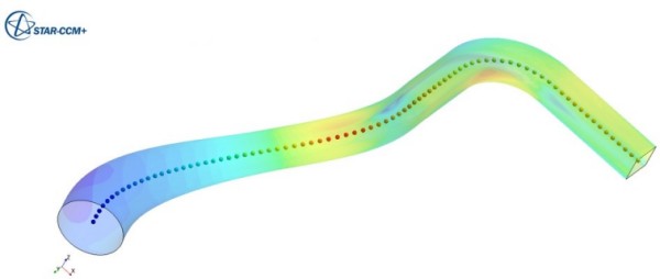
Given a report configuration: Reports > group_1 > group_2 > rep_name, rep_name.getParent() returns Reports (with the class ReportsManager). There is a Java Macro to get the direct parent group (in this case group_2) available at community.sw.siemens.com/s/question/. ./how-to-get-the-group-of-an-object-with-java-api
A Java macro to run multiple cases by changing rotation speeds can be found at community.sw.siemens.com/s/article/Java-macro-to-run-multiple-rotational-speeds-and-save-multiple-sim-files-in-a-single-run
Java macro that removes all reports: community.sw.siemens.com/s/article/How-to-remove-all-the-reports-in-a-sim-file-with-minimal-number-of-clicks-using-a-java-macro
Report number of geometry parts, regions, boundaries and interfaces in a sim file: community.sw.siemens.com/s/article/How-to-find-number-of-parts-regions-boundaries-and-interfaces-using-macro-and-save-the-info-as-text-file
Set mass-flow-inlet type boundary condition by reading strings and double values from each row in a .csv file: community.sw.siemens.com/s/article/Set-Boundary-Condition-for-multiple-boundaries-using-a-Java-Macro
Create Sphere and Mesh It:
  MeshPartFactory meshPartSphere = sim_1.get(MeshPartFactory.class);
  SimpleSpherePart spherePart = meshPartSphere.createNewSpherePart(sim_1.get(SimulationPartManager.class));
  spherePart.setDoNotRetessellate(true);
  LabCoordinateSystem labCS_sph = sim_1.getCoordinateSystemManager().getLabCoordinateSystem();
  spherePart.setCoordinateSystem(labCS_sph);
  Coordinate origin_sph = spherePart.getOrigin();
  origin_sph.setCoordinateSystem(labCS_sph);
  origin_sph.setCoordinate(units_sph, units_sph, units_sph, new DoubleVector(new double[] {0.0, 0.0, 0.0}));
  // Set location of sphere center (x0, y0, z0) in units defined by units_sph
  origin_sph.setValue(new DoubleVector(new double[] {sph_x0, sph_y0, sph_z0}));
  spherePart.getRadius().setUnits(units_sph);
  // Set sphere radius in units defined by units_sph
  spherePart.getRadius().setValue(sph_r);
  spherePart.getTessellationDensityOption().setSelected(TessellationDensityOption.MEDIUM);
  spherePart.rebuildSimpleShapePart();
  spherePart.setDoNotRetessellate(false);
Import STL Mesh and Generate Volume Mesh
  Units un_mm = (Units) sim_1.getUnitsManager().getObject("mm"));
  un_mm.setPreferred(true);
  PartImportManager partImportManager_0 = sim_1.get(PartImportManager.class);
  partImportManager_0.importStlPart(resolvePath(STL_File_Name),
    "OneSurfacePerPatch", units_1, true, 1.0E-5);

  Region region_0 = sim_1.getRegionManager().createEmptyRegion();
  region_0.setPresentationName("Fluid_Region");
  Boundary boundary_0 = region_0.getBoundaryManager().getBoundary("Default");
  region_0.getBoundaryManager().removeBoundaries(new
    NeoObjectVector(new Object[] {boundary_0}));
  FeatureCurve featureCurve_0 = (FeatureCurve) region_0.getFeatureCurveManager()
    .getObject("Default");
  region_0.getFeatureCurveManager().removeObjects(featureCurve_0);
  FeatureCurve featureCurve_1 = region_0.getFeatureCurveManager()
    .createEmptyFeatureCurveWithName("Feature Curve");
  MeshPart meshPart_0 = (MeshPart) sim_1.get(SimulationPartManager.class)
    .getPart("Fluid_Domain");
  sim_1.getRegionManager().newRegionsFromParts(new NeoObjectVector(new Object[]
    {meshPart_0, spherePart}), "OneRegion", region_0, "OneBoundaryPerPartSurface",
    null, "OneFeatureCurve", featureCurve_1, false);

  MeshContinuum mshCon = sim_1.getContinuumManager().createContinuum(MeshContinuum.class);
  PhysicsContinuum pc_1 = sim_1.getContinuumManager().createContinuum(PhysicsContinuum.class);
  mshCon.enable(ResurfacerMeshingModel.class);
  mshCon.enable(DualMesherModel.class);
  mshCon.enable(GenCylModel.class);
  // Use trimmer (Cartesian or Cut-cell) mesh
  mshCon.enable(TrimmerMeshingModel.class);
  mshCon.enable(PrismMesherModel.class);
  // Set base size
  mshCon.getReferenceValues().get(BaseSize.class).setValue(baseSize);
  ResurfacerMeshingModel resurfMesh = mshCon.getModelManager()
    .getModel(ResurfacerMeshingModel.class);
  resurfMesh.setDoCompatibilityRefinement(true);
  resurfMesh.setDoAutomaticSurfaceRepair(false);

  MaxTrimmerSizeToPrismThicknessRatio trimmerToPrismRatio =
    mshCon.getReferenceValues() .get(MaxTrimmerSizeToPrismThicknessRatio.class);
  trimmerToPrismRatio.setLimitCellSizeByPrismThickness(true);
  SizeThicknessRatio sizeThicknessRatio_0 = trimmerToPrismRatio.getSizeThicknessRatio();
  // Prism to field thickness ratio and Number of boundary layers
  sizeThicknessRatio_0.setNeighboringThicknessMultiplier(prism_field_ratio);
  NumPrismLayers numBL = mshCon.getReferenceValues().get(NumPrismLayers.class);
  numBL.setNumLayers(n_BL);
  PrismThickness prismHt = mshCon.getReferenceValues() .get(PrismThickness.class);
  prismHt.getRelativeOrAbsoluteOption().setSelected(RelativeOrAbsoluteOption.ABSOLUTE);
  GenericAbsoluteSize genAbsSize = (GenericAbsoluteSize) prismHt.getAbsoluteSize();
  // Set relative size
  GenericRelativeSize rel_size_prism = (GenericRelativeSize) prismHt.getRelativeSize();
  rel_size_prism.setPercentage(50.0);

  Units un_inch = (Units) sim_1.getUnitsManager().getObject("in");
  genAbsSize.getValue().setUnits(un_inch);
  genAbsSize.getValue().setValue(h_BL);
  PrismLayerStretching prism_stretch = mshCon.getReferenceValues() .get(PrismLayerStretching .class);
  prism_stretch.setStretching(1.5);

  // Specify curvature refinement number of points around a circle
  SurfaceCurvature refineCurvature = mshCon.getReferenceValues().get(SurfaceCurvature.class);
  SurfaceCurvatureNumPts n_refineCurvature = refineCurvature.getSurfaceCurvatureNumPts();
  n_refineCurvature.setNumPointsAroundCircle(n_curve_refine);

  // Surface growth rate (ratio of triangle sizes)
  SurfaceGrowthRate surfaceGrowthRate_0 = mshCon.getReferenceValues()
    .get(SurfaceGrowthRate.class);
  surfaceGrowthRate_0.setGrowthRate(rate_surf_growth);
  SurfaceSize surfaceSize_0 = mshCon.getReferenceValues().get(SurfaceSize.class);
  RelativeMinimumSize relMinSize = surfaceSize_0.getRelativeMinimumSize();

  // Set triangle minimum size percentage
  relMinSize.setPercentage(miz_size_perc);
  SimpleTemplateGrowthRate growthRate = mshCon.getReferenceValues()
   .get(SimpleTemplateGrowthRate.class);
  // Set volume mesh and nearfield growth rates (FAST, MEDIUM, SLOW, VERYSLOW)
  growthRate.getGrowthRateOption().setSelected(GrowthRateOption.SLOW);
  growthRate.getSurfaceGrowthRateOption()
   .setSelected(SurfaceGrowthRateOption.VERYSLOW);

  // Remove existing feature curves
  region_0.getFeatureCurveManager().removeObjects(featureCurve_1);

  MeshPipelineController meshPipelineController =  sim_1.get(MeshPipelineController.class);
  meshPipelineController.initializeMeshPipeline();

  SurfaceRep surfaceRep_0 = (SurfaceRep) sim_1.getRepresentationManager()
    .getObject("Initial Surface");

  Boundary boundary_1 = region_0.getBoundaryManager().getBoundary("bnd_name_1");
  Boundary boundary_2 = region_0.getBoundaryManager().getBoundary("bnd_name_2");
  Boundary boundary_3 = region_0.getBoundaryManager().getBoundary("bnd_name_3");
  boundary_3.setBoundaryType(FreeStreamBoundary.class);

  // Identify feature curves using angle criteria 'feature_angle'
  FeatureCurve featureCurve_2 = surfaceRep_0.createFeatureEdgesOnBoundaries(
    new NeoObjectVector(new Object[] {bnd_name_1, bnd_name_2, bnd_name_3}),
    true, true, true, true, true, true, feature_angle, false);

  SurfaceSizeOption surfaceSizeOption_2 = featureCurve_2.get(MeshConditionManager.class)
    .get(SurfaceSizeOption.class);
  surfaceSizeOption_2.setSurfaceSizeOption(true);
  SurfaceSize surfaceSize_2 = featureCurve_2.get(MeshValueManager.class).get(SurfaceSize.class);
  RelativeMinimumSize relativeMinimumSize_2 = surfaceSize_2.getRelativeMinimumSize();

  // Set feature curve minimum size
  relativeMinimumSize_2.setPercentage(min_mesh_perc);
  RelativeTargetSize relativeTargetSize_2 = surfaceSize_2.getRelativeTargetSize();
  relativeTargetSize_2.setPercentage(edge_tgt_perc);

  SurfaceSizeOption surfaceSizeOption_3 = boundary_3.get(MeshConditionManager.class)
    .get(SurfaceSizeOption.class);
  surfaceSizeOption_3.setSurfaceSizeOption(true);
  SurfaceSize surfaceSize_3 = boundary_3.get(MeshValueManager.class).get(SurfaceSize.class);
  surfaceSize_3.getRelativeOrAbsoluteOption().setSelected(RelativeOrAbsoluteOption.ABSOLUTE);
  AbsoluteMinimumSize absoluteMinimumSize_3 = surfaceSize_3.getAbsoluteMinimumSize();

  // Set triangle size
  absoluteMinimumSize_3.getValue().setValue(min_tria_size);
  AbsoluteTargetSize absoluteTargetSize_3 = surfaceSize_3.getAbsoluteTargetSize();
  absoluteTargetSize_3.getValue().setValue(tria_size);

  // Generate mesh and save SIM file
  if (bool_surf_mesh) {
    meshPipelineController.generateSurfaceMesh();
    sim1.getSceneManager().createGeometryScene("Mesh Scene", "Outline", "Mesh", 3);
    Scene scene_surf_mesh = sim_1.getSceneManager().getScene("Mesh Scene 1");
    scene_surf_mesh.initializeAndWait();
  }
  if (bool_volm_mesh) meshPipelineController.generateVolumeMesh();
  if (bool_save_mesh) sim_1.saveState(resolvePath(sim_file_name));
Check and Look-ups
Check if a physics continuum already existsPhysicsContinuum pc_lookup = lookupObject(PhysicsContinuum.class);
if (pc_lookup != null) {
notifyUser("Continuum " + pc_lookup.getPresentationName + " already exits");
return;
} else {
notifyUser("A physics continuum is required to proceed.");
return;
}
Region region_x = lookupObject(Region.class);
region_x.setContinumm(pc_lookup);
// Add the continuum to loopup list
addToTaskLookup(pc_lookup);
SingleComponentLiquidModel liquid_mat = pc_1.getModelManager() .hasModel(SingleComponentLiquidModel .class);
if (liquid_mat == null) {
  return false;
}
Material water = liquid_mat.getMaterial();
if (! (water instanceOf Liquid)) {
  return false;
}
MaterialProperty mat_prop = (Liquid) water).getMaterialProperties()
  .hasObjectOfClass(PolynomialDensityProperty .class .getName();
if (mat_prop == null) {
  notifyUser("Material property is not a polynomial function.");
  return false;
}
MaterialPropertyMethod mat_prop_method = mat_prop.getMethod();
if (!(mat_prop_method instanceOf TemperaturePolynomial)) {
  notifyUser("Material property is not a function of temperature");
  return false;
}
Check if a boundary name is defined or not
public boolean CheckBoundaryNames(GeometryPart part) {
  partFound = false;
  for (PartSurface surf : part.getSurfaces()) {
    if("inlet".equals(surf.getPresentationName())) {
      partFound = true;
    }
  }
}
Arrays: Range of Variables
RangeMultiValue range_start_end = planesection.getRangeMultiValue();
range_start_end.setNValues(4);
range_start_end.getStartQuantity(10.0);
range_start_end.getStartQuantity().setUnits(un_mm);
range_start_end.getEndQuantity(20.0);
range_start_end.getEndQuantity().setUnits(un_mm);

DeltaMultiValue range_delta = planesection.getDeltaMultiValue();
range_delta.setNValues(4);
range_delta.getStartQuantity(10.0);
range_delta.getStartQuantity().setUnits(un_mm);
range_delta.getDeltaQuantity.setValue(5.0);
range_delta.getDeltaQuantity().setUnits(un_mm);
Specify parameters using an input file
Use an *.ini file which can contain several command line options, one option per row. Rows starting with the "#" symbol are treated as comments. The parameter names in the command line option must match the parameter names in the simulation set-up *.sim file. For example:#Specify geometry -param geomStep .\Projects\Manifold.stp # Specify Boundary Conditions -param mass_flow_rate 1.5kg/s -param inlet_temperature 300C -param wallFlux 250.0W/m^2 -param HTC 10.0W/m^2/K -param TREF 40.0C
Get the bounding box of visible object(s) where the computeVisibleBounds returns an array of (maxx, minx), (maxy, miny), (maxz, minz). You can return an Array by using .toArray() instead of .toString(). Ref: community.sw.siemens.com/how-to-get-a-parts-enclosing-box-vertices-using-a-macro
Scene currentScene = sim_1.getSceneManager().getScene("Outlets");
sim_1.println(currentScene.getDrawableScene().computeVisibleBounds().toString());
Alternatively, the two corners of boundaing box can be accessed using:
SimpleBlockPart simpleBP = (SimpleBlockPart) sim_1.get(SimulationPartManager.class).getPart("Block");
DoubleVector Corner_1 = simpleBP.getCorner1().getSIValue();
DoubleVector Corner_2 = simpleBP.getCorner2().getSIValue();
The content on CFDyna.com is being constantly refined and improvised with on-the-job experience, testing, and training. Examples might be simplified to improve insight into the physics and basic understanding. Linked pages, articles, references, and examples are constantly reviewed to reduce errors, but we cannot warrant full correctness of all content.
Template by OS Templates