- CFD, Fluid Flow, FEA, Heat/Mass Transfer
Tune-in to GNU OCTAVE
MATLAB-compatible OCTAVE Scripts, Example Solutions of ODE / Set of ODEs
Numerical Solutions, Optimization

Table of Contents
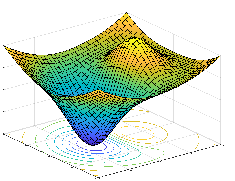
Quadratic Optimization - sqp [+] Root of a non-linear equation of one variable |:| Linear Programming - glpk |:| Solution of a set of ODE [:] Travelling Wave on StringsNumerical solutions with GNU OCTAVE is presented for transient heat transfer, mechanical vibrations, motions of slider crank mechanism, system of ODE, motion of a projectile with viscous drag, optimization using Least-Squares Optimization, Linear Programming and Sequential Quadratic Programming (SQP) methods to name few applications.
OCTAVE can be used to solve partial differential equations and set of ordinary differential equations numerically. This is a great tool where user do not have to write any code, just specify the boundary and initial conditions. However, there is certain process which needs to be followed such as a higher order ODE needs to be converted into a set of linear ODE.
OCTAVE scripts are highly [but reasonably not 100%] compatible to MATLAB. Few of the examples on this page are adaptation of MATLAB codes available in book "Mechanical Vibrations" by Singiresu S. Rao. The code "as provided" in book was initially run in OCTAVE and error / warning messages in OCTAVE were rectified. In addition some improvisation was carried out such as vectorization of calculation to eliminate for loops as far as possible.
Additionally, this page contains numerical solutions using OCTAVE in heat transfer, mechanical vibrations, animation of motions of mechanisms such as slider crank, projectile with viscous drag, animation of travelling wave on string.
A comparison of OCTAVE with other programs is summarized below:| Feature | OCTAVE | FORTRAN | C | JAVA |
| Case-sensitive | Y | N | Y | Y |
| Comment | % | C, ! | /* ... */ | // |
| End of Statement | ; | Newline character | ; | ; |
| Line Continuation | ... for statement \ for strings | Any character | \ | Not required |
| Variable Definition* | x = 1; No explicit definition | real x = 1 | real x = 1; | real x = 1; |
| If Loop | if ( x == y ) x = x + 1; endif | if (x .EQ. y) then x = x + 1 endif | if (x = y) { x = x + 1; } | if (x = y) { x = x + 1; } |
| For Loop | for i=0:10 x = i*i; ... end | DO loop | for (i=0; i<= 10, i++) { ... } | for (i=0; i<= 10, i++) { ... } |
| Arrays | x(5); 1-based | x(5) 1-based | x[5]; 0-based | x[5]; 0-based |
| File Embedding | File in same folder | include "common.dat" | #include "common.h"; | import common.class; |
* by default numeric constants are represented within Octave by double precision floating-point format
Difference between a function file and script file
Excerpts from user manual: Unlike a function file, a script file must not begin with the keyword function. If it does, Octave will assume that it is a function file and that it defines a single function that should be evaluated as soon as it is defined. A script file also differs from a function file in that the variables named in a script file are not local variables, but are in the same scope as the other variables that are visible on the command line. Even though a script file may not begin with the function keyword, it is possible to define more than one function in a single script file and load (but not execute) all of them at once. To do this, the first token in the file (ignoring comments and other white space) must be something other than function.
Quadratic Optimization - sqp
Most of the optimization problems have 5 components:- Objective Function - the method to quantify the required performance of the design quantitatively. This is the dependent variable and the main function which needs to be minimized or maximized as the case may be.
- Control Variables - these are the independent variables which can (usually need to) vary in a pre-determined ranges such as size, material, cost...
- Bounds - as stated above, optimization is a close-ended process and the variables usually have both lower / upper bounds or at least one bound - lower or upper. This bounds needs to be specified based on experience or common sense.
- Design constraints - this refers to the dependency of one control variables with others. For example, the maximum value of fillet radius at a step will depend on the step height.
- Performance constraints - it needs to be considered while defining the objective function. For example, optimization of a pipe diameter will require to keep the maximum velocity below a certain value to avoid erosion which will further depend on material selection.
Redirect OCTAVE output to a File: use diary utility. diary("output.log"); octave_script.m; diary off;
% Optimization of area of a gear train for given "GEAR RATIO" & "centre distance"
%
%                  , * * ,                  , * * * ,
%               ,*         ^              *           *
%      , , ,   *             *           *             *
%    *      ` *               *         *               *
%   *        **               *   ....  *   		    *   n gears
%   *        **               *         *               *
%    *      *  *             *           *             *
%       ^ ^      *         *               *          *
%                  ^ * * *                   ^ * * *
%
% Number of gears in gear train
  n = 6;
%
% Define lower bound of the gear radius which is > 0
  loBnd(:) = 0;
%
% Define upper bound of the gear radius < centre distance between first and last
  upBnd(:) = 25;
%
% phi  = @(x) pi*sum(x(1)^2 + x(2)^2 + ... + x(n)^2);
% Minimise area of the gear trains which is [pi*sum of square of radii]. Note x is
% vector of variable size and is defined by size of initialization vector x0
  objFun = @(x) sumsq(x);
%
% Constraint equation for gear ratio R1/R2 * R2/R3 * ... * Rn_1/Rn = R1/Rn = GR
  g1 = @(x) x(1) - 2*x(end);
%
% Constant equation for centre distance: R1 + D2 + D3 + ... + Dn_1 + Rn = 10
% that is R1 + 2R2 + 2R3 + ... + 2Rn_1 + Rn = 10
  g2 = @(x) x(1) + 2*sum(x(2:(end-1))) + x(end) - 10;
%
% Combine the two constraint equation as array of equations.
  g  = @(x) [g1(x); g2(x)];
%
% Initialize x-vector as gears of uniform radii = Centre distance/number of gears
  dr = 10/n;
  x0 = dr(ones(1,n));
%
% Use Successive Quadratic Programming (sqp) solver
% x = sqp(x0, objFun, g, [])
  x = sqp(x0, objFun, g, [], loBnd, upBnd)
%
% Check for centre-distance with optimized radii
  x(1) + 2*sum(x(2:(end-1))) + x(end)
Linear Regression
Download OCTAVE/MATLAB file from here. Given N measurement points, the curve fit of the form y = m*x + c is the value of m and c which minimize the total squared error. Thus, the method of curve-fitting or regression analysis is also an optimization problem.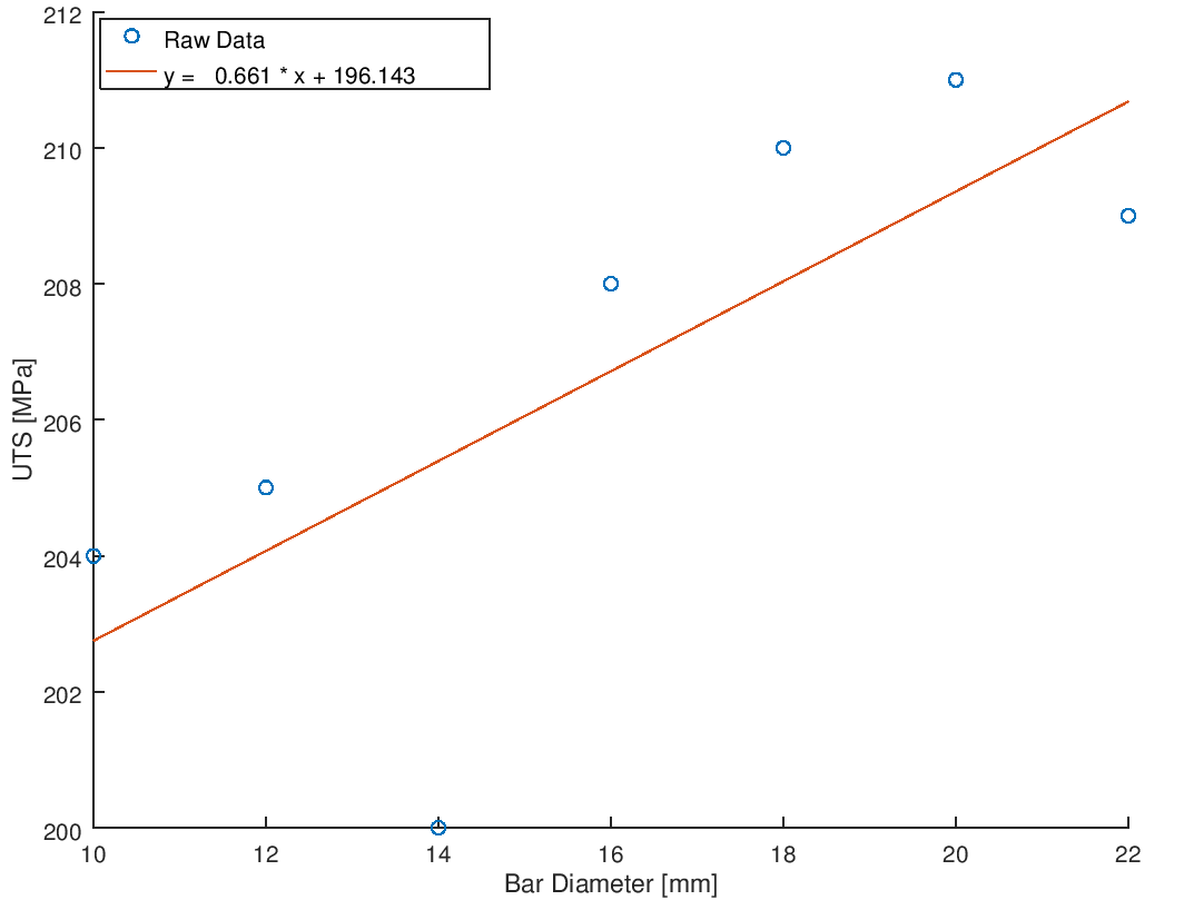
Root of a non-linear equation of one variable
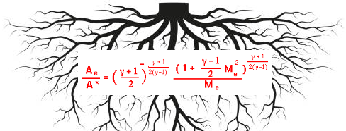
  k = 1.40;          #Gas constant
  A_As = 2.0;        #A/A*
  %
  A = (k-1)/(k+1);
  B = (A_As)**(2*A);
  %
  % Define non-linear function: f(x) = A*Ma*Ma - B*Ma^(2A) + 2/k+1 = 0
  f = @(x) A * x**2 - B * x**(2*A) + 2.0/(k+1.0);
  % Initial guess: note that the two roots will be in the range Ma < 1.0 and Ma > 1.0
  Ma1 = fsolve (f, 0.1)
  Ma2 = fsolve (f, 5.0)
The values are: Ma1 = 0.3059, Ma2 = 2.1972. The calculation of area-ratio for a given Mach number is straightforward as described below.
A_As = (1/Ma) * ((1+(k-1)/2 * Ma^2) / (k/2+0.5))^((k/2+0.5)/(k-1));The vectorized version is as follows:
A_As = (1./Ma) .* ((1+(k-1)/2 * Ma.^2) / (k/2+0.5)).^((k/2+0.5)/(k-1));
Normal shock relation for Mach number downstream of a shock is given by:
Ma_Y = sqrt((Ma_X.^2 + 2/(k-1)) / ((2*k/(k-1))*Ma_X.^2 - 1));
Linear Programming - glpk
% Maximize F = 2x1 + 3x2 + 4x3       subject to
%   3x1 + 2x2 - x3  <=  50
%  -2x1 + x2 - 4x3  >= -80
%   3x1 + x2 + 2x3  <=  100
%   xi >= 0,  i = 1, 2, 3
clc; clear;
% Cost coefficients
  c = [2, 3, 4]';
%
% Matrix of constraint coefficients
  A = [3, 2, -1;   -2, 1, -4;   3, 1, 2];
%
% The right hand side of constraints
  b = [50, -80, 100]';
%
% Lower bound for the design variables
  lb = [1, 0, 0]';
%
% Upper bound for the design variables
  ub = [20, 30, 40];
%
% Constraint type: U and L indicate inequalities with upper and lower bound
% respectively, S indicates equality constraint
  ctype = "ULU"
%
% Variable type: C is for continuous (real number), I for Integer
  vartype = "CCC";
%
% Minimization or Maximization? if 1, it is minimization; if -1, it is maximization
  s = -1;
%
% Set parameters for computation
% Level of messages output by solver. 3 is full (verbose) output. Default is 1.
  param.msglev = 3;
%
% The limit on number of simplex iterations
  param.itlim = 10;
%
% Let OCTAVE find the Optimal solution
% glpk function is the one that solves the Linear Programming (LP) problem.
  [xmin, fmin, status, extra] = glpk(c, A, b, lb, ub, ctype, vartype, s, param);
%
% Print output the solution ot Octave console (terminal)
  xmin
  fmin
Solution of a set of ODE
As mentioned earlier, OCTAVE can be used to solve set of ODE with ease. However, it requires some special representations as explained in the example below.
% Solver system of 2 ODE in OCTAVE. Note that the system of equations having
% order higher than 1 needs to be converted into a system of linear ODE. E.g.
%
% Here q denotes theta
% d^2[q1]/dt^2 = -Keq/J1 * (q1 - q2)
% d^2[q2]/dt^2 = -Keq/J2 * (q1 - q2)
% -----------------------------------------------------------------------------
% OCTAVE solves the system on linear ODE expressed as row vector.
%
% Convert the variables q1 & q2 as well as their first derivatives as row vector
% Let q(1) = q1, q(2) = d[q1]/dt, q(3) = q2, q(4) = d[q2]/dt
%
% Thus, the system of second order order ODEs containing two equations are
% converted to first order ODE containing 4 equations. Note, the RHS of these
% equations will form SET of ODEs to be solved.
% 1) q(1) = q1,     d[q1]/dt   =  q(2)
% 2) d^2[q1]/dt^2 = d[q(2)]/dt = -Keq/J1*(q(1) - q(3))
% 3) q(3) = q2,     d[q2]/dt   =  q(4)
% 4) d^2[q2]/dt^2 = d[q(3)]/dt =  Keq/J2*(q(1) - q(3))
%
clc; clear;
%------------------------------------------------------------------------------
J1 = 5; J2 = 3;
Keq = 100;
%
% Initialize value of q1, d[q1]/dt, q2 and d[q2]/dt as COLUMN VECTOR
q0 = [0.0; 0.0; 0.04; 0.0];
%
% Define the set of linear ODE as column vector using ANONYMOUS function method
% Note that only ODE should be part of the array
f = @(t, q) [q(2); -Keq/J1*(q(1) - q(3)); q(4); Keq/J2*(q(1) - q(3))];
%
% Define time-span of solution
t = [0: 0.01: 5.0];
%
% Solve system of equation:  ODE23 (non-stiff problem) / ODE45 (stiff problems)
% Output is as column vector: x-axis as time axis and y-axis as variables
[t, qa] = ode45(f, t, q0);
%------------------------------------------------------------------------------
% Plot results: Remember we have defined 4 variables by 4 different linear ODE.
% Hence qa is a two dimension array with 4 columns & number of rows defined by
% number of time steps. qa(:, 1) is the angular displacement - q1, qa(:, 3) is
% the angular displacement q2.
%
subplot(211)
plot(t, qa(:, 1));
%
% Add titles for the plot and axes
title('\theta_1(t)');   xlabel('t'), ylabel('\theta_1');
% Format X-axis ticks
xtick = get (gca, "xtick");
xticklabel = strsplit (sprintf ("%.2f\n", xtick), "\n", true);
set (gca, "xticklabel", xticklabel)

% Format Y-Axis ticks
ytick = get (gca, "ytick");
yticklabel = strsplit (sprintf ("%.3f\n", ytick), "\n", true);
set (gca, "yticklabel", yticklabel);
%
subplot(212)
plot(t, qa(:, 3));
%
% Add titles for the plot and axes
title('\theta_2(t)');   xlabel('t'), ylabel('\theta_2');
% Format X-axis ticks
xtick = get (gca, "xtick");
xticklabel = strsplit (sprintf ("%.2f\n", xtick), "\n", true);
set (gca, "xticklabel", xticklabel)

% Format Y-Axis ticks
ytick = get (gca, "ytick");
yticklabel = strsplit (sprintf ("%.3f\n", ytick), "\n", true);
set (gca, "yticklabel", yticklabel);
Travelling Wave on Strings
This script takes few user inputs and calculates the mode shape. The mode shape is plotted at different time steps which can be captured as gif animation or a movie file. The video of wave travel and transverse vibration of string is shown below. The slow motion video demonstrates how energy is transferred from left to right.
% Animation of a traveling wave on string - fixed at one end:
% y(t, x) = A*sin(w*t - k*x) or y(t, x) = A * sin(w * [t - x/v])
% -----------------------------------------------------------------------------
  clear; clc;
%
% Length [m], velocity [m/s], Amplitude [m]
  L = 1.00;
  v = 5.00;
  A = 0.10;
% Mode of vibration: 1 = Fundamental mode, 2 = First overtone or mode-2, so on
  n = 2;
%
% Number of sub-divisions on string
  x = [0: L/50: L];
%
% Wavelength: L = n * lambda, nu = v / lambda = w / 2 / pi
  lambda = L / n;
  nu     = v / lambda;
  w      = 2 * pi * nu;
  T      = 1 / nu;
% Time interval and time steps
  t = [0: T/20: 5*T];
%------------------------------------------------------------------------------
str = strcat('Travelling wave mode - ', num2str(n));
for i = 1 : length(t)
  % Calculation vertical positions y(x)
  y = A * sin(w .* (t(i) - x ./ v));

  plot(x, y, "linestyle", "-", "linewidth", 1, 'o', "color", 'k');
  title(str);   xlabel('x [m]'); ylabel('y [m]');
  %axis("equal");
  set (gca (), "ylim", [-A*2, A*2]);
  % Format X-axis ticks
  xtick = get (gca, "xtick");
  xticklabel = strsplit (sprintf ("%.2f\n", xtick), "\n", true);
  set (gca, "xticklabel", xticklabel);

  % Format Y-Axis ticks
  ytick = get (gca, "ytick");
  yticklabel = strsplit (sprintf ("%.2f\n", ytick), "\n", true);
  set (gca, "yticklabel", yticklabel);

  pause (T/20)
end
Projectile Motion: with and without Air Drag
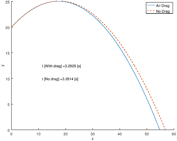
% Animation of a projectile: with and without air drag
% -----------------------------------------------------------------------------
  clear; clc;
%
% Angle of projection [rad]
  q = pi/6;
%
% Initial velocity of projection [m/s]
  V0 = 20;
%
% Initial height of projection [m]
  Y0 = 20;
%
% Acceleration due to gravity [m/s^2]
  g = 9.81;
%------------------------------------------------------------------------------
% Calculation for "No Wid Drag" case
  t_fl = V0/g * sin(q) + 1/g * sqrt((V0*sin(q))^2 + 2 * g * Y0);
  tspan = [0: 0.001 : t_fl*5];
%
  V0x = V0 * cos(q);
  x0 = [0; V0x];
%
  V0y = V0 * sin(q);
  y0 = [Y0; V0y];
%
% Define stopping criteria
% opt = odeset ("OutputFcn", @projectileDragFunX, "RelTol", 1e-6);
  opts = odeset('Events', @projectileStop, 'OutputFcn', @odeplot);
  [t, y] = ode45('projectileDragFunY', tspan, y0, opts);
%
% For debuggin purposes: check t-y plot
% plot(t, y(:, 1));   xlabel('x');   ylabel('y');
%
  tn = length(t) - 1;
  dt = t(end) / tn;
  tspan = [0: dt : t(end)];
  [t, x] = ode23('projectileDragFunX', tspan, x0);
%
% Clear the y-t plot generated by odeplot defined with OutputFcn
  clf reset;
%
% Plot x-y data for projectile motion with drag
  hold on;
  plot(x(:,1), y(:, 1));   xlabel('x');   ylabel('y');
  ylim([0 max(y(:,1))]);
%
% Reset time span for projectile motion without drag
  tspan = [0: 0.005 : t_fl];
  Xt = V0 .* cos(q) .* tspan;
  Yt = Y0 + V0 .* sin(q) .* tspan - 1/2 .* g .* tspan.^2 ;
  plot(Xt, Yt, "linestyle", "--", "linewidth", 1);
%
  annoText = strcat('t [With drag] = ', num2str(t(end)), ' [s]');
  text (max(Xt(:))/5, max(Yt(:))/2.0, annoText);
  annoText = strcat('t [No drag] = ', num2str(t_fl), ' [s]');
  text (max(Xt(:))/5, max(Yt(:))/2.5, annoText);

  legend('Air Drag', 'No Drag');
  hold off;
  print -dpng projectile.png -color -landscape;
%
% Optionally print flight duration in the terminal window
  disp ("The time of flight with air drag:"), t(end)
  disp ("The time of flight without air drag:"), t_fl
%-----=-----=-----=-----=------=-----=-----=-----=-----=-----=-----=-----=-----
function fx = projectileDragFunX (t, x)
  fx = zeros(2, 1);

  % Acceleration due to gravity [m/s^2]
  g = 9.81;
  %
  % Wind drag coefficient [-], reference area [m^2] and density of air [kg/m^3]
  Cd  = 1.2;
  A   = 0.001;
  rho = 1.185;
  %
  % Mass of the projectile in [kg]
  m   = 0.5;
  %----------------------------------------------------------------------------
  fx(1) = x(2);
  fx(2) = -1/2/m * Cd * A * rho * x(2)^2 * sign(x(2));
end
%-----=-----=-----=-----=------=-----=-----=-----=-----=-----=-----=-----=-----
function fy = projectileDragFunY (t, y)
  fy = zeros(2, 1);

  % Acceleration due to gravity [m/s^2]
  g = 9.81;
  %
  % Wind drag coefficient [-], reference area [m^2] and density of air [kg/m^3]
  Cd  = 1.2;
  A   = 0.001;
  rho = 1.185;
  %
  % Mass of the projectile in [kg]
  m   = 0.5;
  %----------------------------------------------------------------------------
  fy(1) =  y(2);
  fy(2) = 0 - g - 1 / 2 / m * Cd * A * rho * y(2)^2 * sign(y(2));

end
%-----=-----=-----=-----=------=-----=-----=-----=-----=-----=-----=-----=-----
function [value,isterminal,direction] = projectileStop(t, y)
% Locate the time when projectile hits the ground and stop integration.
% Check for y = 0
  value = y(1) + 0.1;
%
% stop the integration
  isterminal = 1;
%
% negative direction
  direction = -1;
end
Response of a Spring-Mass-Damper system under Base Excitation
This example demonstrates use of ODE23 function and solution of inhomogeneous linear differential equations 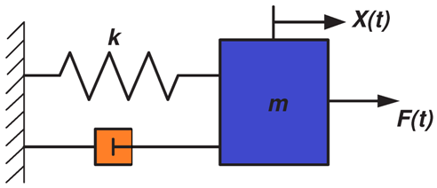
% This program will use the function baseExc_Fun.m, they should be in the same folder
%
% Following statement refers to row vector {0.0 0.2 0.4 0.6 ... 5.0}
  tspan = [0.0 : 0.02 : 2.0];

  x0 =    [0; 0.1];
  [t,x] = ode23('baseExc_Fun', tspan, x0);
  disp('      t         x(t)     xd(t)');
  disp([t x]);
  plot(t,x(:,1));
  xlabel('t');
  ylabel('x(t)');

% Annotations in plot: 'gtext' does not work in OCTAVE. text(x, y, 'x(t)'); is equivalent feature.
% However, gtext is used to place text on the current figure using the mouse and hence warning
% message might be due to incorrect handling of the script.

% Instead 'legend' feature can be used.

  legend('x(t)');
  title('Response under Base Excitation');
% baseExc_F.m
function f = baseExc_Fun(t,x)
f =    zeros(2,1);
m =    100;
k =    500;
z =    0.50;
w =    10.0;
Y0 =   0.05
f(1) = x(2);

% ... is used to continue statement on next line [similar to _ in Excel vba]
f(2) = k/m*Y0*sin(w*t) + sqrt(k*m)*w* Y0*cos(w*t)/m ...
    - sqrt(k*m)/m *x(2) - (k/m)*x(1);
Root Locus Plot
% Load packge to solve controls equation [if not already loaded]
  pkg load control;
% G(s) = [N0*s^n + N1 *s^(n-1) + ... + Np] / [D0*s^m + D1 *s^(m-1) + ... + Dq]
  clf

% num = [ N0 N1 N2 ... Np ]; - Note the coefficients are in decreasing order of power of s
%                            - Only one element = no 's' term, just DC gain term
  num = [5];

% den = [ D0 D1 D2 ... Dq];  - Note the coefficients are in decreasing order of power of s

  den = [100 5  1 0];

%-----------------------------------------------------------------
% This extra statement makes it compatible to both MATLAB & Octave
  sys= tf(num, den);
%-----------------------------------------------------------------

% rlocus(num, den) directly works in MATLAB but not in Octave
  rlocus(sys);
Go to top
Free Vibration Response of Spring-Mass-Damper System
% Free vibration response to under-damped system
  m  =   10;        k  =   1000;
  c  =   25;        %Critical damping ratio = 2*sqrt(k*m) = 200
  x0 =   0.01;      v0 =   0.20;    tspan = [0: 0.01 : 2.0];
  [x, xd, xdd] = underDamped_Fun(m, k, c, x0, v0, tspan);
  subplot(231)
  plot(tspan, x);   xlabel('t');   ylabel('x(t)');
  subplot(232)
  plot(tspan, xd);  xlabel('t');   ylabel('dx/dt');
  subplot(233)
  plot(tspan, xdd); xlabel('t');   ylabel('d^2x/dt^2)');

 % Free vibration response to underdamped system
  c = 250;
  [x, xd, xdd] = overDamped_Fun(m, k, c, x0, v0, tspan);
  subplot(234)
  plot(tspan, x);   xlabel('t');   ylabel('x(t)');
  subplot(235)
  plot(tspan, xd);  xlabel('t');   ylabel('dx/dt');
  subplot(236)
  plot(tspan, xdd); xlabel('t');   ylabel('d^2x/dt^2)');

%a From OCTAVE user guide - plot with 2x3 grid will have as follows:
%
% +-----+-----+-----+
% |  1  |  2  |  3  |
% +-----+-----+-----+
% |  4  |  5  |  6  |
% +-----+-----+-----+

% Under-damped system
function [x, xd, xdd] = underDamped_Fun(m, k, c, x0, v0, dt);
  %x0 = x(t=0), v0 = dx/dt|t=0
  % x = x(t), xd(t) = dx/dt = v(t), xdd = d^2x/dt^2 = a(t)

  wn = sqrt(k / m);                 % Natural frequency
  ccrit = 2.0 * sqrt(k * m);        % Critical damping factor
  zeta = c / ccrit;                 % Damping ratio
  wd = sqrt(1.0 - (zeta^2))*wn;     % Damped natural frequency

  C1 = x0;                          % Constants of integration
  C2 = (v0 + zeta * wn * x0)/wd;
  CC = sqrt(C1^2 + C2^2);
  phi = atan(C1 / C2);

  x   =  CC .* exp(-zeta .* wn .* dt) .* sin(wd .* dt + phi);
  xd  =  CC .* exp(-zeta .* wn .* dt) .* (wd .* cos(wd .* dt + phi) - zeta .* wn .* sin(wd .* dt + phi));
  xdd = -(c .* xd + k .* x) ./ m;

% Critically-damped system
function [x, xd, xdd] = critDamped_Fun(m, k, c, x0, v0, dt);
  %x0 = x(t=0), v0 = dx/dt|t=0
  % x = x(t), xd(t) = dx/dt = v(t), xdd = d^2x/dt^2 = a(t)

  wn = sqrt(k / m);                 % Natural frequency
  C1 = x0;                          % Constants of integration
  C2 = (v0 +  wn * x0);

  x   =  (C1 + C2 .* dt) .* exp(-wn .* dt);
  xd  = -wn .* x + (v0 + wn .* x0) .* exp(-wn .* dt);
  xdd =  wn.^2 .* x;

% Over-damped free vibration - no external excitation
function [x, xd, xdd] = overDamped_Fun(m, k, c, x0, v0, dt);
  %x0 = x(t=0), v0 = dx/dt|t=0
  % x = x(t), xd(t) = dx/dt = v(t), xdd = d^2x/dt^2 = a(t)

  wn = sqrt(k / m);                 % Natural frequency
  ccrit = 2.0 * sqrt(k * m);        % Critical damping factor
  zeta = c / ccrit;                 % Damping ratio
  wd = sqrt(1.0 - (zeta^2))*wn;     % Damped natural frequency

  C1 =  x0/2 * (zeta * wn /wd + 1) + v0/2/wd;
  C2 = -x0/2 * (zeta * wn /wd - 1) - v0/2/wd;
  x1 = -zeta + sqrt(zeta^2 -1); x2 = -zeta - sqrt(zeta^2 -1);

  x   =  C1 .* exp(x1 .* wn .* dt) + C2 .* exp(x2 .* wn .* dt);
  xd  =  C1 .* x1 .* wn .* exp(x1 .* wn .* dt) + ...
         C2 .* x2 .* wn .* exp(x2 .* wn .* dt);
  xdd =  C1 .* x1.^2 .* wn^.2 .* exp(x1 .* wn .* dt) + ...
         C2 .* x2.^2 .* wn^.2 .* exp(x2 .* wn .* dt);
The plot of results from the script is shown in following figure: 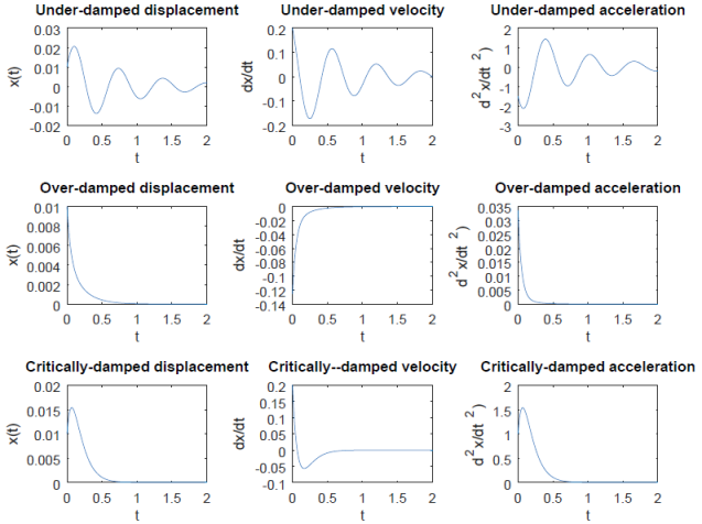
Go to top
Spring-Mass-Damper System - Numerical Solution: ODE32
% Free response under varying damping coefficient: zeta = 0.1, 1.0 and 2.0
  m   =   10;
  k   =   1000;
  c   =   25;    %Critical damping ratio = 2*sqrt(k*m) = 200
  xt0 =   0.01;
  vt0 =   0.20;
  tspan = [0: 0.01 : 2.0];

  % ---------------------------------------------------------------------------
  % mx'' + cx' + kx = F(t), F(t) = 0 for free vibration
  % x(1)  = x,  x(2) = x'  -> x'' = x''(1) = x'(2)
  % x'(2) = F(t)/m - k/m * x - c/m * x' = F(t) /m - k/m * x(1) - c/m * x(2)
  %                                                      ^^^^^         ^^^^^
  %                                                     x(1)=x       x(2)=dx/dt
  % f(1) = dx/dt = x' = x(2)
  % f(2) = d^x/dt^2 = x'' = x'(2) = F(t) /m - k/m * x(1) - c/m * x(2)
  %----------------------------------------------------------------------------
  x0 = [xt0; vt0];

  zeta = 0.1;     %zeta = c / Ccrit = c / 2 / sqrt(k*m)
  c = zeta * 2 * sqrt(k*m);
  g =  @(t, x)  [ x(2); (-k/m .* x(1) - c/m .* x(2) )];
  [t, x] = ode23(g, tspan, x0);
  subplot(331)
  plot(t, x(:, 1));   xlabel('t');   ylabel('x(t)');
  grid on;  % should be placed only after the plot command
  title('Displacement - Underdamped');
  subplot(332)
  plot(t, x(:, 2));   xlabel('t');   ylabel('dx(t)/dt');   grid on;
  title('Velocity - Underdamped');
  subplot(333)
  a = (-k/m .* x(:, 1) - c/m .* x(:, 2) );
  plot(t, a);   xlabel('t');   ylabel('d^2x(t)/dt^2');   grid on;
  title('Acceleration - Underdamped');

  zeta = 1.0;     %zeta = c / Ccrit = c / 2 / sqrt(k*m)
  c = zeta * 2 * sqrt(k*m);
  g =  @(t, x)  [ x(2); (-k/m .* x(1) - c/m .* x(2) )];
  [t, x] = ode23(g, tspan, x0);
  subplot(334)
  plot(t, x(:, 1));   xlabel('t');   ylabel('x(t)');    grid on;
  title('Displacement - Critically-damped');
  subplot(335)
  plot(t, x(:, 2));   xlabel('t');   ylabel('dx(t)/dt'); grid on;
  title('Velocity - Critically-damped');
  subplot(336)
  a = (-k/m .* x(:, 1) - c/m .* x(:, 2) );
  plot(t, a);   xlabel('t');   ylabel('d^2x(t)/dt^2');   grid on;
  title('Acceleration - Critically-damped');

  zeta = 2.0;     %zeta = c / Ccrit = c / 2 / sqrt(k*m)
  c = zeta * 2 * sqrt(k*m);
  g =  @(t, x)  [ x(2); (-k/m .* x(1) - c/m .* x(2) )];
  [t, x] = ode23(g, tspan, x0);
  subplot(337)
  plot(t, x(:, 1));   xlabel('t');   ylabel('x(t)');     grid on;
  title('Displacement - Overdamped');
  subplot(338)
  plot(t, x(:, 2));   xlabel('t');   ylabel('dx(t)/dt'); grid on;
  title('Velocity - Overdamped');
  subplot(339)
  a = (-k/m .* x(:, 1) - c/m .* x(:, 2) );
  plot(t, a);   xlabel('t');   ylabel('d^2x(t)/dt^2');   grid on;
  title('Acceleration - Overdamped');
The plot of results from the script is shown in following figure: 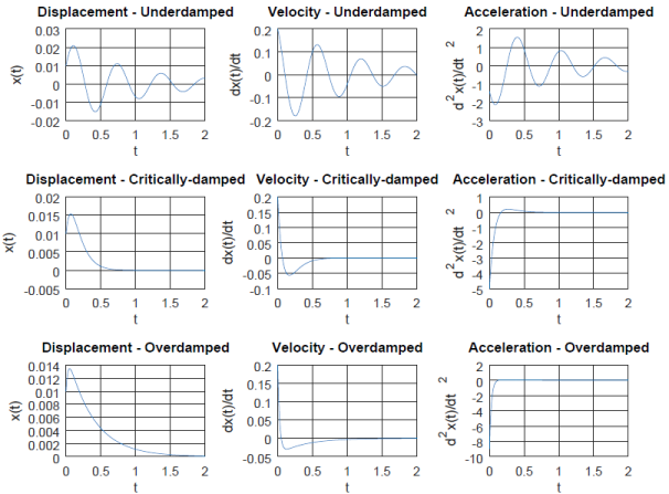
Go to top
Flow Rate vs. Pressure Drop Curve for Simple Pipe
clc
clear
%  Define constants
e   = 0.0005;      % Surface roughness [m]
D   = 0.050;       % Hydraulic diameter [m]
rho = 1.185;       % Density [kg/m^3]
nu  = 1.21e-5;     % Kinematic Visosity[m^2/s]

Q   = [0.005:  0.005:  0.050];    % Flow rate in [m^3/s]
% Check for correct definition of Q_0, dQ and Q_n
% If (Q_n - Q_0) / dQ != Integer, exit with warning message

L   =  10;  	   % Length along flow direction[m]
%------------------------------------------------------------------------------
% Define friction factor implicit formula as in-line function

for i = 1 : size(Q, 2)
  V   = Q(i) / (0.25 * pi * D^2);       % Velocity in m/s
  Re  = D * V / nu;                     % Reynolds number at each flow rate

  % Note that Re is changing every iterations, hence the function needs to be
  % re-defined every iteration to calculate f at new Rey-number
  ff = @(f) 1 / sqrt(f) + 2 * log10(e / D / 3.7 + 2.51 / Re / sqrt(f));
  fric = fzero(ff, [0.01 0.20]);

  dP(i) = fric * L / D * (1/2 * rho * V^2);
end

plot (Q .* 1000, dP, "linestyle", ":", "linewidth", 2, "marker", 'o');
xlabel('Q [L/s]');
ylabel('dP [Pa]');

% Format X-axis ticks
  xtick = get (gca, "xtick");
  xticklabel = strsplit (sprintf ("%.1f\n", xtick), "\n", true);
  set (gca, "xticklabel", xticklabel)

% Format Y-Axis ticks
  ytick = get (gca, "ytick");
  yticklabel = strsplit (sprintf ("%.1f\n", ytick), "\n", true);
  set (gca, "yticklabel", yticklabel);
The plot of results from the script is shown in the following figure: 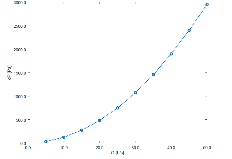
Go to top
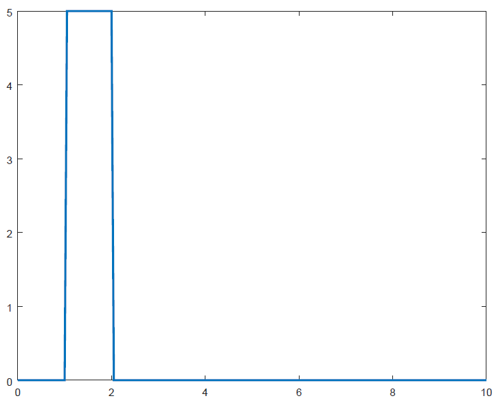
Generate Square Pulse - Analogous to Heavyside Function
clc
clear
  x1 = 1.0;  x2 = 2.0;  Fs = 5.0;
  x = [0.0 : 0.05 : 10];
  F = max(sign(x - x1), 0) .* Fs - max(sign(x - x2), 0) .* Fs;
plot(x, F, "linewidth",  2);
The plot of results from the script is shown below.
Go to top
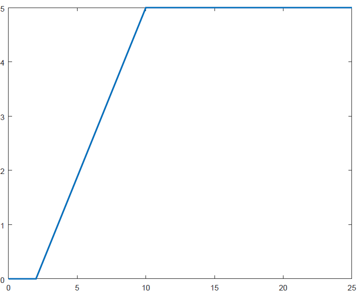
Generate Ramped-Step Pulse
clc
clear
  x1 =   2.0;  x2 =  10.0;  y2 =   5.0;
  x = [0.0 : 0.05 : 25];   % Note x(end) should be >= x3

  F1 = max(sign(x - x1), 0) .* y2 ./ (x2 - x1) .* (x - x1);
  F2 = max(sign(x - x2), 0)  .* y2 ./ (x2 - x1) .* (x - x1);
  F3 = max(sign(x - x2), 0)  .* y2;

  F = F1 - F2 + F3;
  plot(x, F, "linewidth",  2);
  set(gca, 'XTick', 0 : 5 : x(end));    %Adjust as per x
  set(gca, 'YTick', 0 : 1 : y2);
The plot of results from the script is shown below.
Go to top
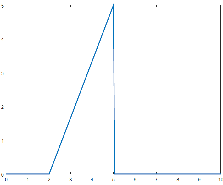
Generate Saw-Tooth Pulse
  x1 =  2.0;   x2 =  5.0;   y2 =  5.0;
  x = [0.0 : 0.05 : 10];

  F1 = max(sign(x - x1), 0) .* y2 ./ (x2 - x1) .* (x - x1);
  F2 = max(sign(x - x2), 0) .* y2 ./ (x2 - x1) .* (x - x1);

  F = F1 - F2;
  plot(x, F, "linewidth",  2);
  set(gca, 'XTick', 0 : 1 : 10);
The plot of results from the script is shown below.
Go to top
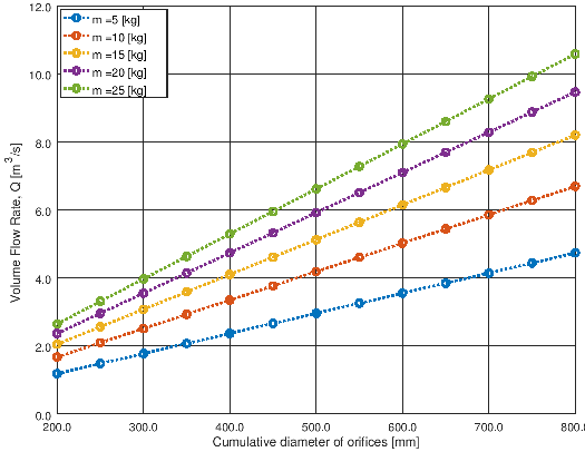
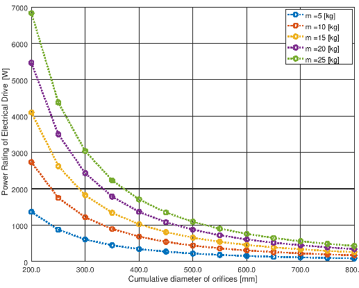
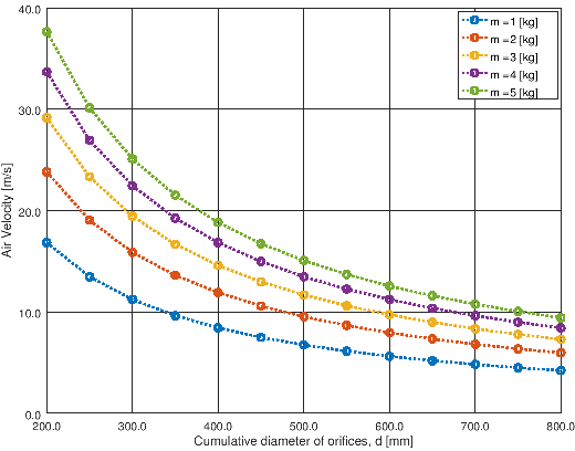
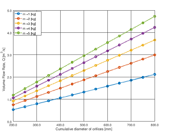
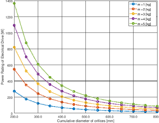
Basic Hydro-dynamic curves - objects floating in air
- This is based on force balance and thrust calculation for order of magnitude analysis. The data has been generated for different masses of the object (say drones) and exit orifice sizes required to generate the upward thrust. The plots of results from the script shown below.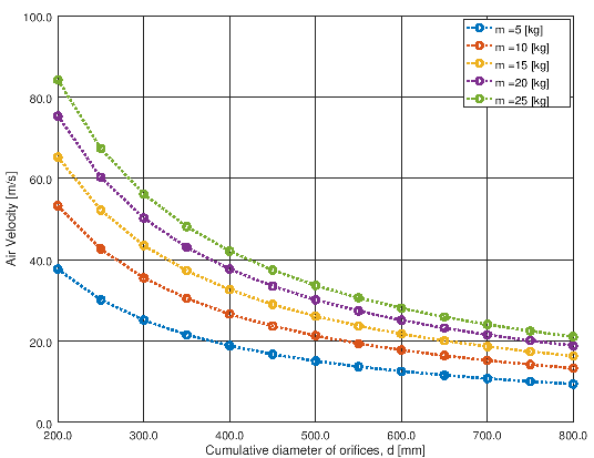
% Air velocity calculation to hold an object hanging in air
%
  clc; clear; clf reset;
%
% Acceleration due to gravity [m/s^2]
  g = 9.81;
%
% Atmospheric pressure [Pa]
  p = 99000;
%
% Temperature [C]
  T = 40;
%
% Gas constant for Air [J/kg.K]
  R = 287;
%
% Static pressure drop from inlet to exit - loss coefficient: dP_s = K/2*rho*V^2
% Entrace, friction and local losses
  K = 0.75;
%
% Hydraulic efficiency of fan / compressor [%]
  eH = 0.60;
%
% Mechanical efficiency of electric motor drive [%]
  eM = 0.95;
%------------------------------------------------------------------------------
% Density of air
  rho = p / R / (T + 273.11);
%
% Dimeter range of the holes (cumulative effective diameter) in [mm]
  d = [200 : 50 : 800];
  legengTxt = cell(length(d), 1);
  i = 1;
%
  for m = [5:5:25]
    Mg = 4 * m * g / pi / rho;
    V = sqrt(Mg ./ (d ./1000).^2);
%
	hold on;
	figure(1);
	%subplot (2, 1, 1);
    plot(d, V, "linestyle", ":", "linewidth", 2, "marker", "o");
    xlabel('Cumulative diameter of orifices, d [mm]');
	ylabel('Air Velocity [m/s]');
    grid on;
    set (gca, "ygrid", "on");
    legendTxt{i} = strcat('m = ', num2str(m), ' [kg]');

    % Format X-axis ticks
    xtick = get (gca, "xtick");
    xticklabel = strsplit (sprintf ("%.1f\n", xtick), "\n", true);
    set (gca, "xticklabel", xticklabel)
    %set (gca, 'xtick', [200 25 800]);

    % Format Y-Axis ticks
    ytick = get (gca, "ytick");
    yticklabel = strsplit (sprintf ("%.1f\n", ytick), "\n", true);
    set (gca, "yticklabel", yticklabel);
	hold all;
	i = i + 1;
  end
  legend(legendTxt);
  print -dpng figure1.png -color -landscape;
  hold off;
%
%------------------------------------------------------------------------------
  i = 1;
  legengTxt2 = cell(length(d), 1);
  for m = [5:5:25]
    Mg = 4 * m * g / pi / rho;
    V = sqrt(Mg ./ (d ./1000).^2);
    Q = pi ./ 4 .* (d ./1000) .^2 .* V;
	hold on;
	figure(2);
	%subplot (2, 1, 2);
    plot(d, Q, "linestyle", ":", "linewidth", 2, "marker", "o");
    xlabel('Cumulative diameter of orifices [mm]');
	ylabel('Volume Flow Rate, Q [m^3/s]');
    grid on;
    set (gca, "ygrid", "on");
    legendTxt2{i} = strcat('m = ', num2str(m), ' [kg]');

    % Format X-axis ticks
    xtick = get (gca, "xtick");
    xticklabel = strsplit (sprintf ("%.1f\n", xtick), "\n", true);
    set (gca, "xticklabel", xticklabel)

    % Format Y-Axis ticks
    ytick = get (gca, "ytick");
    yticklabel = strsplit (sprintf ("%.1f\n", ytick), "\n", true);
    set (gca, "yticklabel", yticklabel);
	hold all;
	i = i + 1;
  end
  legend(legendTxt2,  "location", 'northwest');
  print -dpng figure2.png -color -landscape;
  hold off;
%
%------------------------------------------------------------------------------
  i = 1;
  legengTxt2 = cell(length(d), 1);
  for m = [5:5:25]
    Mg = 4 * m * g / pi / rho;
    V = sqrt(Mg ./ (d ./1000).^2);
    Q = pi ./ 4 .* (d ./1000) .^2 .* V;
%
	dPs = K ./2 .* rho .* V.^2;
	dPv = 1 ./2 .* rho .* V.^2;
	dP = dPs + dPv;
%
%   Hydraulic power required to hold it in air
    JH = Q .* dP ./ eH;
%   Net power required to hold it in air
    JM = JH ./ eM;

	hold on;
	figure(3);
	%subplot (2, 1, 2);
    plot(d, dP, "linestyle", ":", "linewidth", 2, "marker", "o");
    xlabel('Cumulative diameter of orifices [mm]');
	ylabel('Power Rating of Electrical Drive [J]');
    grid on;
    set (gca, "ygrid", "on");
    legendTxt2{i} = strcat('m = ', num2str(m), ' [kg]');

    % Format X-axis ticks
    xtick = get (gca, "xtick");
    xticklabel = strsplit (sprintf ("%.1f\n", xtick), "\n", true);
    set (gca, "xticklabel", xticklabel)

    % Format Y-Axis ticks
    ytick = get (gca, "ytick");
    yticklabel = strsplit (sprintf ("%.0f\n", ytick), "\n", true);
    set (gca, "yticklabel", yticklabel);
	hold all;
	i = i + 1;
  end
  legend(legendTxt2,  "location", 'northeast');
  print -dpng figure3.png -color -landscape;
  hold off;
The charts for mass range 1 [kg] to 5 [kg] will like like shown below.
The content on CFDyna.com is being constantly refined and improvised with on-the-job experience, testing, and training. Examples might be simplified to improve insight into the physics and basic understanding. Linked pages, articles, references, and examples are constantly reviewed to reduce errors, but we cannot warrant full correctness of all content.
Template by OS Templates