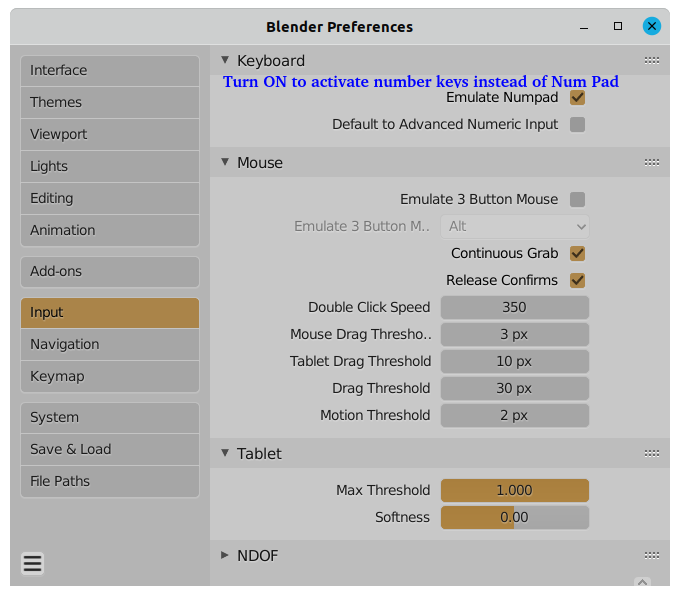
- CFD, Fluid Flow, FEA, Heat/Mass Transfer
Geometry Cleanup
Solution Domain
Geometry or computational domain for CFD simulation requires a water tight geometry with simplification to handle the mesh creation process. Solution of computational domain refers to 2D or 3D geometry in which fluid flow and/or heat transfer phenomena need to be solved. This is known as "ZONES" in FLUENT, "REGIONS" in STAR-CCM+ and "DOMAIN" in CFX. These are "volumes surrounded by closed surfaces(called boundaries)" in 3D and "areas closed by edges or lines (called boundaries)" in 2D. It is the mesh and nodes generated to define and represent the physical space mathematically. No geometrical information is associated with the solution domain.
Geometry Clean-up Steps [+] Checklist for Computational Domain [*] Dimensional Values to be Recorded {*} Defeaturing in ANSYS Discovery |:| Values to record about computational domain [+] Blender for Geometry Clean-up |+| Create Periodic Planes |:| Domain size reduction by sub-modeling ]=[ CAD Data Exchange [=] Parametric Geometry Creation [*] Recommendations for Parametric Modeling [=] Create Driving Dimension using Measurements from within the Pull Tool ]*[ Objects, Selections and Named Selections |=| Setting Colour of Faces |+| Power Selection {*} Creating cylinders by extruding surfaces }={ External Connections (:) Remove all chamfers and rounds |\/| Basic Operations: Open - Save - Import |/\| Remove - Translate - Copy Holes \:/ Create Fluid Volume [?] Get and Set Dimension Values
Scripting in ANSYS Discovery [*] Script to move objects defined by Named Selections |+| Scripting in ANSYS DesignModeler {*} CATIA VBA [+] SOLIDWORKS Summary (+) STEP File Format [=] Check Interfaces or Contacts (*) Smart Selection [*] Create Named Selections [+] Select all rounds and fillets (+) Get bounding box {+} Get centroid of all bodies defined in Named Selection {*} Create named selection based on volume {=} Geometry Editing in FreeCAD
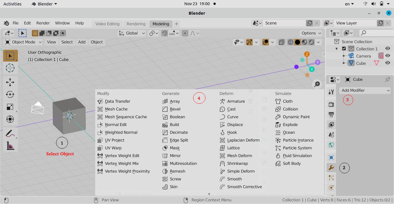
The geometry creation for CFD can be accomplished by either of the following two methods:
- Create geometry in any CAD (Computer-Aided Design) software such as Unigraphics, Catia, Pro/E, Solidedge. The geometry information created so far is called to be in "Native CAD" format. This geometry should be translated to a Neutral format such as IGES, STEP, Parasolid. All Pre-processors available has build-in capacity to read (Import) CAD data in this format. Once the geometry is imported into the Pre-processor, defeature as per requirement.
- The second approach is to create geometry directly into the pre-processor. All commercial pre-processors has basic built-in features to create Geometrical Entities. We strongly recommend this approach for following two cases:
- 2D simulation
- When geometry is axisymmetric. In this case, one needs to create the 2D cross-section first and then extrude it by rotation. In ANSYS FLUENT, in the axisymmetric model the boundary conditions should be such that the centerline (where the radius reduces to zero) is an axis type instead of a symmetry type. The axis should the z-axis. Thus, for all 2D simulations, FLUENT expects geometry to be in XY-plane.
- One widely used term in numerical simulation is Topology. A precise explanation is provided by Georgios Balafas in his master's thesis for the Master of Science program in Computational Mechanics "Polyhedral Mesh Generation for CFD-Analysis of Complex Structures": The topology of a mesh is an abstraction of the geometric model, that provides unambiguous, shape independent information about the relation between the entities that form the mesh structure. To this end, a mesh database is used in order to store various-level attributes of entities of different dimensions. These typically include 0-D entities, referred to, in literature, as vertices or nodes, 1-D entities, referred to as edges, 2-D entities, referred to as faces or facets and 3-D entities, referred to as solids, volumes, regions or cells.
- Few other definition taken from previous reference:
- "A face is said to be classified on the boundary of the geometric model, when it is adjacent to only one solid, which means that the free side of the face forms an external boundary. In the opposite case, where a face is adjacent to two solids, it is classified in the interior of the geometric model."
- Mesh edges inherit their classification by their adjacent faces. Specifically, when an edge has at least one adjacent face that is classified on a model's boundary surface, the edge is also classified on the same boundary. To be more precise, in a conforming non-manifold three-dimensional mesh, an edge will have either zero or at least 2 adjacent boundary faces, however detecting one of them can be considered enough to classify the edge on the boundary as well. Furthermore, when an edge's adjacent boundary faces are classified on different boundary surfaces of the model, this denotes the edge's classification on a model's boundary edge, where 2 of its boundary surfaces intersect.
- It is, therefore, adequate to count the amount of different boundary identifiers that are assigned to the adjacent faces of an edge, in order to conclude whether this edge is internal (zero boundary identifiers), on a boundary surface (one identifier), on a boundary edge (2 identifiers), or is a non-manifold edge (> 2 identifiers).
- Extending the aforementioned classification criteria for vertices, a mesh vertex is classified on a model's boundary surface, when at least one of its adjacent edges is also classified on a boundary surface. Additionally, when at least one of the adjacent edges of a vertex is classified on a model's boundary edge, then the vertex is also classified on the same boundary edge. Finally, when there exist at least two adjacent edges classified on two different model's boundary edges, the vertex is classified on a model's corner, formed at the intersection of the boundary edges. In other words, the classification of a vertex with respect to the model can be determined by counting the amount of different boundary identifiers assigned to the adjacent faces of the vertex.
- Zero boundary identifiers denote an internal vertex, while vertices on a boundary surface have adjacent faces with a unique identifier. Nodes on model's boundary edges have adjacency relationships to faces of two boundary identifiers in total and vertices on a model's corner sum up with three adjacent boundary identifiers. Finally, when a vertex has adjacent faces classified to more than three different boundary surfaces, the vertex is non-manifold.
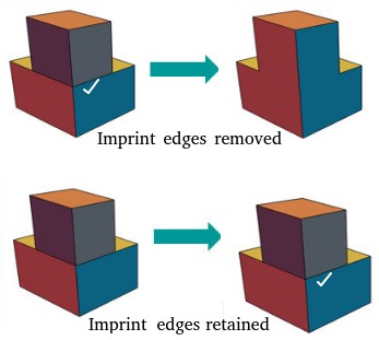
Other operations include: extract centrelines (to plot variation of pressure or temperature vs. position), create mid-planes (to create plots on a non-planar surface), save curve data into .csv file, create enclosure, merges faces, create body-of-influence (BOI) geometry, create Face of Influence (FOI) geometry, scale-up or down a body... ANSYS Discovery has option to create Curve Tables and Hole Tables (Curve Table in the Annotation group under Detail tab), the centreline of a tube can be generated using 'Extract' tool in Beam section under Prepare tab. Fill Surface: create surfaces from free edges of a hole in a facet sheet body, Sew Sheet bodies: combine or sew multiple facet bodies into a single body, Bridge surface: (similar to loft operation in some CAD tools) create a body between two sets of edges of existing facet bodies. Extruding surfaces and sketches directly up to any user defined Plane with the "Up to Plane" method. Keep or delete imprinted edges when uniting bodies.
Creation of post-processing planes: when computational domain is not aligned to coordinate axes or the flow path are curved and twisted that any section would result in multiple non-contiguous surfaces, it is strongly recommended to create post-processing planes during geometry creation and meshing process. These faces should be named with prefix 'post_' and set as internal type in meshing (so that boundary layers do not grow over them). Though most of the solvers and post-processors has option to import such surfaces in STL format and imprint on the mesh, it is time consuming and may result in interpolation error. The 'internal' zone created shall have faces and nodes aligned on it and the solution variables are directly available there to calculate derived parameters such as mass flow rate and pressure. In case of imprinted surfaces, the solution variables have to be interpolated from nearest nodes, face and cell centers.
Unit Systems
Every designer needs to work on length units and thus all CAD modeling program or tool have some built-in features for default units and ways to convert from one units to others. The following image describes options to select unit system in SCDM.
All tools dealing with virtual geometry and mesh generation has option to scale the model. As units are not mentioned at every numerical value, scaling changes the value as per units specified. For example, for a cylinder the tool may contain information 'mm' in header row and only numbers for diameter, length and other key points (nodes, vertices...). When user changes the units to 'm', those values has to be divided by 1000 while only the header gets changed from 'mm' to 'm'.
Checklist for Computational Domain
This step shall not only help in reducing the errors, it will help expedite the simulation activities and shorten lead time. Here the checklist is presented as instructions and not as questions.- Check for symmetry or periodicity in the domain - this is specially helpful when adaptive mesh refinement is required
- After clean-up activity, record the macro parameters such as number of bodies, number of contact surfaces - this is required to match the number of cells zones in mesh
- In ANSYS discovery script editor: print(GetRootPart().GetAllBodies().Count) shall print the number of bodies, or
- use Ctrl+A to select all bodies and the count is shown in the status bar at the bottom
- Create named selections which are easy to identify: for applying boundary layers settings, creating monitor points and post-processing. Note on Encapsulated Surfaces: If a surface body is completely inside a solid body, Share Topology treats it as part of that solid, effectively merging it during simulation**.
- Add prefixes or suffixes to bodies and components for heat sources, special material types and surface parameters (such as emissivity and roughness)
- Split surface where BOI (Body of Influence) or FOI (Face of Influence) needs to be applied (such as downstream the orifices)
- Ensure the FOI surface physically passes through or is in close proximity to the volume to be refined
- Must check: proximities- this issue cannot be easily corrected in pre-processors
- Remove features which are redundant (such as extra lines on curved surfaces)
- Merge small entities - edges, surfaces and if possible bodies too
- Rename the native and source files (Discovery, STEP, CATIA...) easy to identify later
- For multiphase flows where geometry is not aligned with coordinate system, create separate zone for patching - required for domain initialization of volume fraction of a phase
- For large assemblies - number of solid bodies > 50, add appropriate counters or identifier for each type to easily count and retrieve them in meshing, solution and post-processing
**: To prevent shared topology, place solids in a component whose Shared Topology property is set to None, and whose parent components also have this property set to None.
Note that free-edges, self-intersection and sometimes highly skewed boundary cells can be easily corrected in mesh generation tools, proximities are the most difficult to handle. Hence, first check the user should make after importing the CAD geometry into pre-processor is to look for proximities and cells with skewness ≥ 0.99.Proximity-based refinements require different mesh sizes for different bodies. Many a time, it is necessity to generate surface meshes separately and assemble them later. In STAR-CCM+ use File > Import > Import Surface Mesh multiple times selecting "Create New Part" for each import. Then use "Combine Parts" tool in the Geometry node to merge them followed by creating a shared region for connected mesh.
Refer to checklist for mesh generation and update geometry appropriately. The checklist for solver settings including Boundary Conditions can be referred here.
Geometry Clean-up Steps
This is the first step of CFD simulations.Pre-requisite: get familiar with the tool and the specific version being used and do not rely on similar features in tools from same product family. ANSYS Discovery which is the successor of SpaceClaim, has many features under different user menu. For example, in ANSYS Discovery the colour of faces and bodies are set using icon in the model tree and not with (right click) context menu. The right click after selection of a body does not give option to set transparency. HUD: Head-Up Display is a new feature which may seem a nuisance to someone new to Discovery. Similarly, V25R2 adds component names as prefix to the Named Selections which confounds the purpose of named selections. Let's take the example of following geometry: 3 bodies names Base, Body_1 and Body_2.
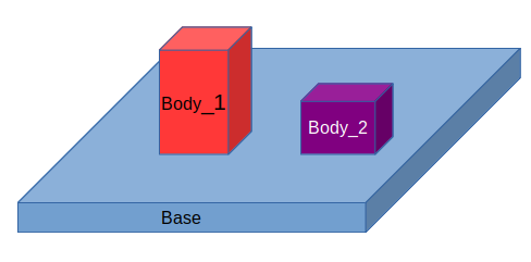
When there is no named selections: face zone names created in FM are base, body_1, body-2, base:body_1, and base_body_2. When the 5 faces each of body_1 and body_2 are put in a Named Selections say ns_bodies, the face zone names created in FM are: base, ns_bodies:body_1, ns_bodies:body_2...
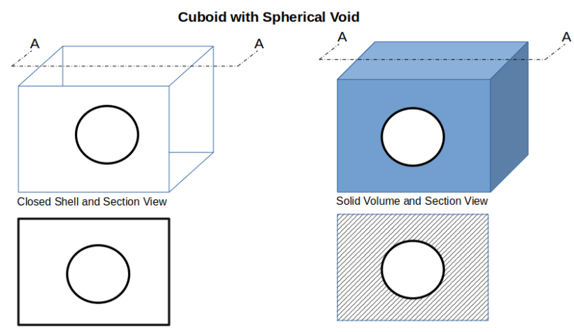
Understanding differences between shell-based (CATIA V5) and solid-based (ANSYS Discovery) representation is important to decide how to transfer CAD data to pre-processor. With shell-based presentation, any section view shows only outline and it does not clearly distinguish material and void regions.
Coming back to geometry defeaturing....
The first step is to know the geometry. If it comprise of sheet metal parts such as fan shroud, it requires handling thin bodies, sharp bends with gap, forming clearance... If the geometry consists of plastic parts, it will have fillets of variable radii and the two adjacent parts may not align properly. The plastic parts usually have lot of ribs and hidden cavities not visible from outside. One trick is to scan through section tool in all three direction and get the insight into the extent and complexity of defeaturing required. This may require 2 to 6 hours.The second step is to organize the geometry into sub-groups easy to handle in batches. This requires moving the bodies into components, renaming them to identify easily. The bodies needs to be grouped into solid, fluid and empty categories. This may take another 2 - 4 hours of effort. Refer to Naming Convention for basic idea.
The third step is deletion of unwanted parts: screws, clips, clamps, body inside another body... and filling cavities, gaps, converting thin sheets to zero-thickness walls or thickening them to get less skewed cells. (Note: If the faces are coloured within the CAD software, SpaceClaim recognizes those colours as "named selections" and transfers them to "Mesh" and "CFX-Pre"). This may take 1 to 2 days based on maturity of the input CAD geometry.The fourth step is to remove small blends (fillets), chamfer, proximities (tangential contact between two curved bodies or a curved face and a flat surface....), extra edges (edges at tangential splits) and combine or segregate bodies into logical groups. Note that removing fillets should always be the last step of defeaturing process. This step may take 4 hours to 2 days.
The fifth step is to save geometry into multiple files based on ease of meshing. Many a times it is better to generate surface mesh into multiple groups and assemble them later especially when there are thin sections such as sheet metal bodies like fan shroud. Sometimes it becomes a necessity to split geometry into extrudable volumes.
The sixth step is to create monitor plane(s) and name them appropriately such as int_mon_fan_up or int_mon_delta_p... This is helpful in case any section surface of the domain creates multiple non-contiguous regions. In ANSYS Fluent, either a clipping operation after surface creation is required or the monitor plane needs to be imported as STL mesh and imprinted in Pre-Post.
Thus, the clean-up activity may take 2 days to 4 days (this excludes mesh generation activity). Note that one may need to iterate between surface mesh and geometry clean-up especially to remove proximities and self-intersections (which may occur despite successful topology sharing). It requires 5 to 10 times more effort to address geometrical challenges inside meshing tool than the CAD tool.Notes:
In ANSYS SpaceClaim, do the Pull operation by isolating the body (that is hiding other bodies). By default, Pull operation shall try to merge all visible objects or those Within same component (otherwise No Merge option needs to be activated for every pull operation). Default behaviour of pull operation: File > Options > Advanced > Pull Tool, in the option "Default Extrude Behavior" select "No Merge".To remove proximity between curved faces, pull the common edge to create a blend or chamfer. Sometimes, merging or collapsing of sliver faces in SpaceClaim is not feasible. These faces can be put into a separate Named Selection (Group) such as ns_sliver_faces utilizing Power Selection feature. Later the boundary elements on these faces can be collapsed in Fluent meshing.
It is better to unite (merge) two bodies than keep them separate (joined) by shared topology. However, this is possible only when the volume occupied by those bodies are empty (void). In case the two bodies cannot be combined (merged), delete the common surfaces (let them be surface bodies than solid bodies) - however such operations should be performed as last step before taking the data to pre-processor.The small gap (such as < 0.2 mm) between solid bodies can be removed by following method in SpaceClaim: select bodies based on power selection of equal volume > hide other bodies > go to Clearance tool section and find out surfaces within 0.2 mm > add the reported surfaces into selection > activate the pull operation > specify the pull distance 0.21 mm.
ANSYS SpaceClaim has a tool named Sharp Edges which highlights edges sharper than the Max edge angle (the angle between normals of faces that share an edge) specified. It has another tool 'Clearance' in the 'Detect' group of the 'Prepare' tab which might be helpful to find out why two bodies cannot be united when they seem to be touching each other.

Make multiple instances independent: sometimes the copies of similar parts are linked and renaming one of them renames all the linked or dependent instances of bodies. In ANSYS Discovery, select all parts, right click and select option Make Independent. This assigns unique ID to all components linked by instance array.
Parts organization is one of the many challenges dealing with large assemblies such as automotive underhood with full car body - this may contain upto 15000 parts or bodies. Sometimes a PCBA may contain more than 500 parts and clear identification is a must as per reference designators. Creating groups or sub-assemblies or components are strongly recommended in such cases. The group name should contain short form of material names and boundary condition type. Refer to the meshing checklist for naming convention. Such convention helps in automation where scripts or macros can search in strings containing sub-strings.
Refer to checklist for mesh generation and update geometry appropriately. Values to be recorded about computational domain - multiple values can be typed separated by comma. Note that it is better to start recording the information to be put in a report from the start rather than preparing the report at the end of the simulation activities.
| S. No. | Description of the Dimension | Value(s) |
| 01 | Orientation (such as direction of gravity) | |
| 02 | Rotation axis (or flow direction) of the fan | |
| 03 | Coordinates of a point on axis of the fan | |
| 04 | Total surface area | |
| 05 | Total volume | |
| 06 | Cross-section area of the inlet(s) | |
| 07 | Cross-section area of the outlet(s) | |
| 08 | Number of fluid-fluid interfaces and names | |
| 09 | Number of fluid-solid interfaces and names | |
| 10 | Number of solid-solid interfaces and names | |
| 11 | Fan hub, tip and shroud diameters | |
| 12 | Thickness and cross-section area of porous domain(s) | |
| 13 | Thickness of printed circuit board and normal direction | |
| 14 | Dimensions of heat sink: thickness, pitch, length, radius |
Parametric Modeling (Geometry Creation) within CFD Environment
For optimization studies, ANSYS Workbench offers options to make simulations in the order defined as DOE (Design of Experiment) table, each row termed as Design Point. ANSYS SpaceClaim and Discovery has option to parametrize the geometrical operations such as Pull, Move... which can be used to change the shape, size and location of bodies. Such activities are specially important in situations where periodicity and symmetry exist such as heat exchangers, fins, external aerodynamics.Parametric Modeling in ANSYS SpaceClaim / Discovery: For all operations which can be parametrized, the symbol 'P' in SpaceClaim and icon within context-menu in Discovery appear to create a parameter. The value field of a parameter can contain basic formula such as 0.02 * 25.4 to convert a dimension from inch to 'mm'.
The Groups tab contains Named Selections, Driving Dimensions and Script Parameters. Driving dimensions can be Measurement, Ruler Dimension, Pattern Count... When a Pull operation is initiated, the option to make it parametric appears only after a value is entered (after pressing the space bar). Similarly, Ruler Dimension can be used to change the size as shown below in one of videos from Ozen Engineering.
"Driving dimensions are created when there is a dimension on screen or a dimension in the properties panel." For example, selecting the round (fillet) and then clicking Create Group in the 'Groups' panel creates a "driving dimension" instead of a "named selection" because the face selected is a round, which has a dimension property that can be controlled from the property panel. Similarly, a "round group" is created each time fill operation is used to create a round (fillet) and is saved in the Filled Rounds folder.
Note: clicking on a driving dimension created with 'Pull' operation automatically activates the 'Pull' operation ↴
Note that the GUI in the two videos are a bit old and in recent versions, Create Group has been replaced with Create NS and Create Parameter. When a dimension is showing and "Create Parameter" is clicked, it usually create a driving dimension with initial value appearing on the screen. The orientation of Move handle can be changed by using the Direction tool guide, holding Alt and selecting a reference object, or by dragging a ball on the axes of the Move handle. That is, Alt + click a point or line orients one of the axes of Move handle towards that point or along that line. Alt+click on a plane, the direction of movement is set perpendicular to the plane. Steps to create Driving Dimensions using Move operation ↴The behaviour of the Move tool changes based on what is selected and direction of axes of move handle change based on the orientation on the screen. Press Ctrl to copy the object selected for movement and place it at the location at which user drags or dimensions the move. Video titled "Using ANSYS SpaceClaim and ANSYS Discovery for Parametric CAD Modeling" from KETIV Technologies gives good explanation of the methods described above. As per help.spaceclaim.com/2016.0.0/en/Content/Groups.htm: Group order is important because they are changed from top to bottom when the change is initiated in an external application.
Steps to create Move handle at 'Zero' initial value is explained below. The yellow centre sphere of Move handle turns into a blue cube when the Move handle is anchored.

- Select face(s) or object(s) to be moved
- Press 'm' or click 'Move' icon under 'Edit' group in Ribbon bar
- Select anchor point or edge
- Select axis on the Move handle
- Press space bar on keyboard ('0' will appear near Move handle origin)
- Click 'Enter' key (to accept '0' as initial value)
- Click on "+Create Parameter" icon in Group tab to create the Driving Dimension.
Move operation is very much similar to Pull operation though the behaviour of the Move tool changes based on what is selected. Though Pull allows operation in only one direction, Move allows operation in multiple directions. If an entire object, such as a solid, surface, or sketch is selected, 'Move' operation translates or rotates the object. If one side of a solid, surface, or sketch is selected, move operation shall enlarge or reduce the size of the object. If an object is moved into another object in the same component, the smaller object is merged into the larger one and receives the larger object's properties. Moving the apex of a cone changes the height, Anchor the Move tool to the outer face to scale the cone.
By default the 'Move' handle seems to be placed at the centroid of chosen objects (faces, edges...). However, there are cases when an axis was create using same set of objects, the location of origin of the axis and location or the origin of move handle were not coincident. In absence of clear documentations, following error may occur.

Create Driving Dimension using Measurements from within the Pull Tool: referenced from User Guide
- Enter the Pull tool and select an object(s) to pull
- Enter the Measure tool (shortcut is e) and measure any single object or measure between two objects
- Click the measurement result that will drive the Pull (hover over measurements output box to display a purple box)
- Once selected, that single measurement will display on screen with arrows pointing to either object chosen for measurement
- Click in the highlighted dimension box and open the Groups panel
- Click "+Create Parameter" and the measurement group gets created.

From Workbench (V20) User Guide: "Negative dimension values can invert the direction vector of operations with which they are associated. This change is applied to the current and subsequent design point updates. As a result, when a Workbench input parameter is used as a driving dimension for a geometry, negative dimension values can result in unexpected geometric changes."
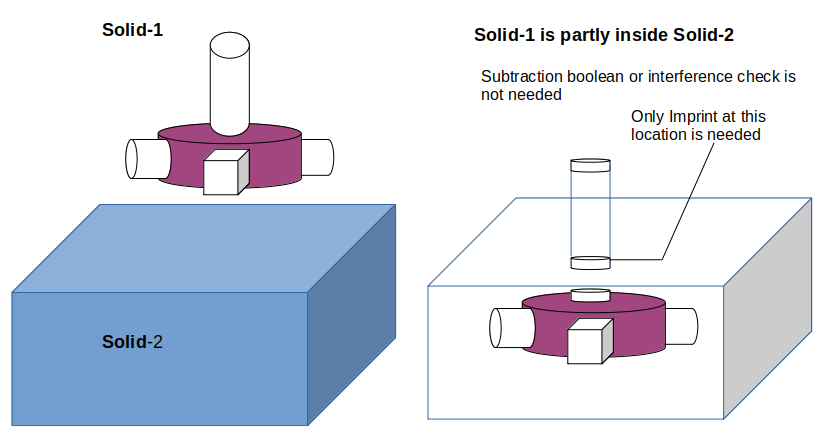
Geometry Fully or Partially Enclosed in a Fluid Domain


It is not explicitly documented in SCDM user manual in which order the parameters get updated - however it is logical to assume that the parameters shall get updated in the order they are created / stored. And the parameters are stored in the order they are created and not in the order sorted by user say ascending alphabetically. It is better to define parameters with constant reference frame instead of taking reference from any other floating object.
ANSYS WB as in version 2024 does not allow to change the ID of parameters though GUI and they are stored in the order they are created. Parameter ID can be changed by editing the Workbench project file *.wbpj using a text editor. Search for all instances of a parameter which usually is named as P** where ** represents the sequence number (such as P1, P2, P13, P21...) and replace them by the new name (preferably keeping the naming convention same). If parameters have been used in expressions, renaming parameters should take care of keeping this dependency.Few Recommendations for Parametric Modeling
- While deciding the mean, low and high levels of parameters: check the design for limiting conditions which may cause manufacturing or assembly limitations
- Keep all references to measure length with respect to fixed surfaces and/or edges (those which are not affected by geometrical changes
- While moving a round (fillet), use the edge of fillet on the side of straight face - in other words align the "direction of move" and "direction of measurement"
- Create parameters in group and order which does not contradict to subsequent constraints - note that if any parameter definition is missed for a shape, it will come later in the list (sequence of update) and may result in incorrect shape and size
- Keep testing the correctness of parametrization in small chunks (such as group of 10 driving dimensions) - this will help identify the driving dimension(s) causing failure in update of the geometry (create back-up after each successful check)
- Create a simple yet distinct naming convention for driving dimensions such p11_x_h where 1 refers to type 1, next 1 refers to item 1, x refers to direction, [h, w, b..] may refer to the variable names such as height, width, gap...
- In ANSYS SpaceClaim, you cannot change the order of driving dimensions - hence a careful planning is critical, especially all the dimensions required for a particular feature such as protrusions or cut-outs should be in consecutive sequence
- Create parameters responsible for changes in size first followed by parameters or ruler dimensions required for translation of objects
- Organize the variables in DOE table in the similar order (as per the expected sequence of update in CAD environment)
- Do not use default location of 'Move' handle which is near the centroid of the chosen objects, if shape changes the centroid will change and hence translation dimension need to account for this change in centroid position.
- Create 10 ~ 20 geometries manually using parameters randomly selected from the DOE table and overlap them in a single file. This will give a good visual representation of expected changes and error / anomaly in parameter values or definitions.
In general (for a single solid body and not assembly), the order of update of parameters or driving dimension should not matter. If the order of update affects the final shape and size of the body, recheck the input dimension - they might not be correct. For example, some update might have resulted in loss of feature (a face or edge) leading to missing reference for next update. "One or more objects may have lost some scoping attachments during the geometry update" or meshing operation get stuck in batch mode (playing a recorded script) > Very often geometry selections such as Named Selections, zones defined for inflation layer settings, reference edge for move operation... become invalid as the edge or surface referred while creating them do not exist at some values of input parameters.
When a parameter is changed in SCDM, the geometry change is updated but the parameter set value does not update in Workbench parameter set. User the option Update Parameter in SpaceClaim under the 'Workbench' tab which will push the updated value to Parameter set.Using an Excel Spreadsheet to Drive Dimensions
This utility is part of add-ins which can be activated using SpaceClaim Options > Add-ins > (Check the box) Excel Dimension Editor Add-in > Restart SpaceClaim.
Driving Changes with Annotation Dimensions
3D annotation dimensions can be used to change design using the Pull and Move tools. Annotation dimensions can be used in combination with ruler dimensions. Dimension can be used for every element in design, from lines in sketches to faces of solids. In Discovery SpaceClaim, dimensions are not constraints rather tools for precise control during the creation or modification of a design. To save a dimension with the design, Ruler Dimension option can be used when pulling or moving.Error: File has wrong dimensions (3) > this is usually reported in case 2D geometry is not in XY plane (which Fluent is expecting). By default SpaceClaim draws sketch in XZ plane which needs to be rotated to meet requirement for Fluent pre-processor.
As per innovationspace.ansys.com/ ... /driving-parameter-and-script-parameter:
# Get list of named selections and driving dimensions in Groups tab
dims_NS = Window.Groups.GetValue(Window.ActiveWindow)
#
# 3-tuple type: value is index 1, type is index 2
# Type = (Linear, Angular, Arc, Area, Diametric, Mass, Volume)
dims_NS[0].TryGetDimensionValue()
dims_NS[0].SetDimensionValue(value)
A script to move objects defined by Named Selection is described below (not tested - generated by AI). Note that SCDM recording feature does not capture steps to create ruler dimensions. And hence the ruler dimensions cannot be accessed in Python script - changing ruler dimension is same as executing a 'Move' operation.
import SpaceClaim.Api.V242 as sc
from SpaceClaim.Api.V242 import Point, Direction, DesignPoint
#from SpaceClaim.Api.V242 import *
'''
User Inputs: Named Selections and Move Direction
object_to_move = Named selection for object(s) to move
move_dir_name  = Named selection of face/edge to get direction
ref_point_name = Named selection of a vertex or point
move_distance  = Distance to move in [mm]
'''
object_to_move = "ns_fillet_x"
move_dir_name  = "ns_mmv_dir_1"
ref_point_name = "ns_ref_pnt_1"
ns_move_anchor = "ns_anchor"
move_distance  = 50

target_selection = Selection.CreateByGroups(SelectionType.Primary, object_to_move)
move_direction = Selection.CreateByGroups(SelectionType.Primary, move_dir_name)
anchor = Selection.CreateByGroups(SelectionType.Primary, ns_move_anchor)
direction = Move.GetDirectionAlignedTo(target_selection, move_direction)
'''
Other options to create direction are:
direction = Move.GetDirectionAlignedTo(anchor, move_direction)
direction = -Direction.DirZ

mv_face = Selection.CreateByGroups(SelectionType.Primary, ns_mv_face) #face normal
direction = Move.GetDirection(mv_face)
'''
options = MoveOptions()
options.CreatePatterns = False
options.DetachFirst = False
options.MaintainOrientation = False
options.MaintainMirrorRelationships = True
options.MaintainConnectivity = True
options.MaintainOffsetRelationships = True
options.Copy = False
options.SnapAssociatedVertices = True
options.SubProportionalRadius = MM(0)
result = Move.Translate(target_selection, direction, MM(5), options) #IN(0.02)
# Note Move calculates 'change' from current value between anchor and target

# Get direction vector from edge or planar face normal
direction_item = move_direction.Items[0]
if direction_item.ShapeType == sc.ShapeType.Edge:
  curve = direction_item.Geometry
  direction_vector = (curve.EndPoint - curve.StartPoint).Direction
elif direction_item.ShapeType == sc.ShapeType.Face:
  face = direction_item.Geometry
  direction_vector = face.Normal
else:
  raise Exception("Move Direction must be an edge or planar face.")

reference_point = Selection.CreateByGroups(ref_point_name)
if reference_point and reference_point.Count > 0:
  ref_item = reference_point.Items[0]
  if hasattr(ref_item, 'Point'):
    ref_point = ref_item.Point
  else:
    ref_point = ref_item.Shape.Geometry.Center
else:
  ref_point = Point.Origin  # default to origin if not specified

move_vector = direction_vector * move_distance
transform = Transform.CreateTranslation(move_vector)

result = Move.Execute(target_selection, transform)
print(f"Moved '{object_to_move}' by {move_distance} along '{move_direction}'")

def getNamedSelection(ns_name):
  select_ns = Selection.CreateByGroups(ns_name)
  if not select_ns or select_ns.Count == 0:
    raise Exception(f"Named Selection '{ns_name}' not found or empty.")
  return select_ns

# Create Driving Dimension as parameter and apply initial transform of 0 [unit]
axis_map = {
  "X": coordinate_system.XDirection,
  "Y": coordinate_system.YDirection,
  "Z": coordinate_system.ZDirection
}
if move_axis not in axis_map:
  raise Exception("Invalid move_axis. Choose from 'X', 'Y', or 'Z'.")
selected_axis = axis_map[move_axis]
end_point = ref_point + 1.0 * selected_axis

initial_transform = Transform.CreateTranslation(selected_axis * 0)
Move.Execute(target_selection, initial_transform)
Get summary of dimensions for edges and/or faces
ns_list = GetActiveWindow() .ActiveWindow .Groups
mea_dim = []
for ns in ns_list:
  if (ns.GetNames().Contains("msr")):
    ns_members = ns.Members
    mea_dim.append(ns_members[0].Shape.Length) # Output is in [m]
mea_dim_row = ','.join(mea_dim)
print(mean_dim_row)
From discuss.ansys.com under topic "Extract edge length and export information":
import os
import io
import json
file_path = os.path.join(r"D:\Projects", "edge_lengths.json")
bodies = GetRootPart().GetAllBodies()
body = bodies[0]
edge = body.Edges[0]
e_length = edge.Shape.Length
len_dict = { "edge length" : e_length }
with io.open(file_path, "w", encoding="utf8") as json_file:
   json.dump(len_dict, json_file, ensure_ascii=False)
Guidelines to Design Thermal Management System
Following considerations are recommended to design air-cooled and liquid-cooled systems:- The available space and envelope such as inlet and outlet connectors, location of fans... should be as per component placement
- For gas (air) cooled systems:
- The design approach with passive cooling (natural convection) and active cooling (forced convection) are different
- Both may use heat spreader (heat sinks) and thermal interface material
- In passive cooling, the orientation of the part and hence the orientation of heat spreader or heat sink should is along direction of gravity
- For active cooling case, the location of fan should be inline with the heat sink and there should be diverging duct to control the swirl of the fans
- For liquid cooled systems:
- First criteria is to meet the pressure drop requirement (maximum permissible pressure drop) for specified flow rate
- The cooling channel should be in a curved or serpentine shape to cover larger surface area which also ensures continuous mixing of hot and cold fluid (no formation of thermal boundary layer)
- The heat conducting face of heat generating devices (MOSFET, IC, Capacitors...) should be directly mounted on the heat sink or cooling channel plates as per the layout of the components
- Ensure good contact between the heat generating parts and the cooling plate or heat spreader by using thermal grease or thermal interface material (TIM)
- The sizing of the channels are iterative: for cooling channels with Aluminium and copper, the liquid (cooling medium) velocity is limited to 2 [m/s] or 5-8 [ft/s]* and for stainless steel the limit is 4 [m/s]. This is to avoid pitting (erosion) at higher liquid velocities. High water velocity in copper channels can strip the protective copper oxide layers and thus accelerate corrosion-erosion of the channels
- Sometimes a minimum average velocity is also need to be met to avoid fouling and depositions on the channel walls
- The minimum wall thickness is governed by burst pressure requirements. In terms of thermal performance, a lower wall thickness leads to better conductive heat transfer.
| Material | Recommended maximum velocity |
| Low Carbon Steel | 10 ft/sec - 3.0 [m/s] |
| Stainless Steel | 15 ft/sec - 4.5 [m/s] |
| Aluminum | 06 ft/sec - 1.8 [m/s] |
| Copper | 08 ft/sec - 2.4 [m/s] |
| 90-10 Cupronickel | 10 ft/sec - 3.0 [m/s] |
| 70-30 Cupronickel | 15 ft/sec - 4.5 [m/s] |
Naming Convention of Boundaries and Cell Zones
In any practical application of CFD simulations, the computational domain may comprise of many cells zones (fluid and solid zones) and boundary zones (walls, inlets and outlets). The engineer responsible for pre-processing may not be the one who creates solver file and post-processes the results. The reviewer(s) of the mesh and simulation set-up will certainly be not the engineer who created them. In order to convey the domain information seamlessly, a naming convention should be adopted, it can be a generic system applicable for large number of projects or a specific system for particular simulation set-up. An example is outlined below with following default setting: Newtonian, stationary, adiabatic, smooth boundaries or zones can be named arbitrarily though it is recommended to chose names and identifiers meaningfully.- Inlet(s) and outlet(s) should be named as b_inlet_id, b_outlet_id where 'id' stands for identifier.
- Walls with boundary conditions (other than adiabatic): w_tpr_id, w_hfx_id, w_htc_id, w_rot_id w_mov_id, w_rgh_id, w_s2s_id where 'rgh' stands for rough walls, s2s stands for coupled solid walls.
- Cell zones: fld_air_id, fld_wtr_id, fld_oil_id, fld_nnw_id, fld_rot_id, por_mom_id, por_thm_id, sld_alm_id, sld_stl_id, sld_src_id ... where 'nnw' stands for non-Newtonian fluids, 'src' stands for solid zones with heat source and/or sink and 'por' stands for porous (fluid) zones.
- Internal planes: int_f2f_id, int_baf_id ... where 'baf' stands for thin walls or baffles.
- Non-conformal interfaces: if_f2f_id, if_s2s_id, if_sta_rot_id, if_por_fld_id, if_por_por_id where 'sta' stands for 'stationary' zones and 'por' stands for 'porous' zones.
- All boundaries with no special setting or conditions to be applied on them can be named as 'b_def_id' or dumy-id1, dumy-id2 or empt-id1, empt-id2 or fblk-id1, fblk-id2 where dumy stands for dummy, empt for empty and fblk for flow-blockers. This is especially important while dealing with assemblies with large number of solids and fluid zones.
DOMAIN SIZE REDUCTION THROUGH SIMILARITY: In order to results of the model to apply to the prototype, strict similarity rules must be followed.
A convenient frame of reference must be defined that applies to both model and prototype and corresponding locations must be defined using dimensionless ratios (for a sphere for example, angle on its surface, longitude and latitude lines). Thus, there exist similar conditions for corresponding points on both model and prototype. That is, the drag coefficient at a particular point on the sphere applies to both model and prototype.
The designer must follow, then geometric similarity (model and prototype), kinematic similarity (velocity vector direction is similar for both model and prototype), dynamic similarity (force vector direction is similar for both model and prototype), thermal similarity (heat fluxes)...
Note that similarity principles cannot be applied for all application without loss of accuracy. For example, to reduce size of an axial flow fan with shroud, either for numerical or experimental investigation, their is no thumb rule to account for blade-tip and shroud clearance. Hence, the designer has to establish his own "quality standards and acceptance criteria" to address this limitation
Domain size reduction by sub-modelling
Domain size reduction by axi-symmetry
Defeaturing in ANSYS Discovery
The pre-processing activities require geometry simplifications (defeaturing) and ANSYS SpaceClaim has some powerful non-parametric features. One of them is the 'Pull' option (short-cut 'p') which is equivalent to 'sweep' or 'extrude' operation. By default, pull direction is tangent to the selected edge or perpendicular to the selected face. A direction can be chosen or pulled (sweep) along a curve. Selection: all holes equal to selected radius, all holes of same radius in same face, all holes of radius equal or smaller than select radius. Blend (b): create surface by two lines (it is equivalent to 'loft' operation in some CAD programs). Fill (f): create surface from a closed loop of curves. Move (m): the 'origin' option is to select the reference point on the source object.
Step-by-Step for Geometry Defeaturing and Simplifications (ANSYS Spaceclaim)
Step-1:
Split the large assemblies into smaller (if possible, geometrically less-dependent) domain. This helps avoid large memory requirement and further geometry clean-up operations as well.Step-2: Re-group and rename the data
The geometry in CAD environment is created keeping in mind the physical construction and assembly sequences. This is not important in mesh generation. It is better to re-group the geometrical (CAD) entities in terms of expected boundary definition. This makes it easy to operate on a smaller section of the entire domain. The selection, hide/unhide and operations such as imprint/ interference become faster.Step-3:
Further segregate the geometry into 'Solids' and 'Surfaces'. This helps chose operations appropriate for the respective category. Such as fillet removal, split, booleans and extrude (pull) is easy on solids.Step-4:
Convert the solids with thin wall thickness into solids with no internal wall and void. For example, a beam with fillets and internal wall.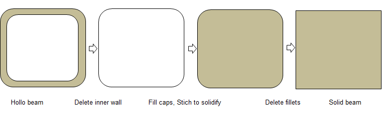
Step-5:
Before removing the wall thickness, use the operations appropriate for solids such as Booleans like unite, intersect... to make sure the once converted to surface, no further operations such as extend /intersection is needed to remove the gaps / connect the surfaces. Note that this method is no recommended for FEA simulation. in CFD the blockage of flow is important where as in FEA the location of centroid is important. 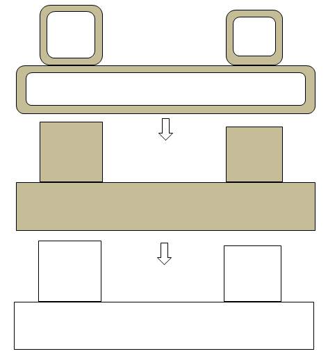
Step-5:
ANSYS Spaceclaim is a CAD-type pre-processor and works better on solids. CFD volume extraction is a analogous to 'negative' of visible solid volumes. Instead of deleted the unwanted surfaces one-by-one, it is recommended and worth trying to create a "bounding box" enclosing the geometry and use a booleaan to subtract the solids from the 'bounding' box. The resultant negative volume of fluid domain is easy to operate and remove the protrusions generated due to gaps in original (input) geometry.SpaceClaim has versatile feature called Pull operation which can be used to extrude faces and edges, create fillets and chamfer and remove materials. Tangent and Natural (curvature continuous) extension can be toggled when dragging the end of a curve. To drag the extension Tangent to the curve, press and hold Ctrl prior to dragging. Press 'Ctrl' and drag to 'Pull' the curve end tangent to the curve. Surface edges can be Pulled normal to their neighbouring face. Press the Ctrl key when you begin the Pull. Press Ctrl and drag to Pull the edge tangent to the surface. Pulling a face with its edges selected extrudes the face without influence from neighbouring faces. Pulling a conical face "Up To" a parallel cylindrical face replaces the cone with the cylinder if the axes are close together. Otherwise, the conical face is replaced with a cylindrical face that is coaxial to the cone and has the same radius as the cylinder.
Tips and Tricks:
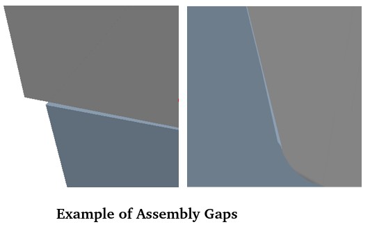
Definition: gaps in the plane of a surface is called lateral (horizontal) gaps and gaps in the direction of area normal is called the transverse (vertical) gap.
If you are dealing with large surfaces with small (transverse) gaps (say < 1% of the biggest geometry or say 1-5 [mm] which you can neglect), follow these steps:
- Create a plane and/or planar surface encompassing the entire geometry which defines the best possible horizontal plane for the lower bound of the geometry.
- Extend (using 'extrude', 'sweep' or 'pull' tool) by amount which covers (fills) all the unevenness (transverse gaps) in the geometry.
- Split the bodies (solid volumes and surfaces) as per appropriate tool. E.g. in ANSYS SpaceClaim, "Split Body" can be used for both solid and surface bodies. 'Split' tool can be used for surfaces only.
- This process will remove the 'local' details such as 'openings', small surfaces or patches for named selection... Project the curves from original geometry as needed and then split the bigger surfaces created during previous operations.
- Delete the unwanted extensions created due to 'extend' and 'trim / split' operations.
- Repeat the process for other bodies in the assembly.
- Repeat the process for the upper and left / right bounds of the geometry. Though, once the lower and upper bounds are flattened (made coplanar), the 'blend' and 'fill' operation can be used to fill any lateral gaps between vertical edges and surfaces.
Fill operation: selecting many contiguous (connected) surfaces for fill operation does not work. However, selecting just one surface out of many makes the 'fill' tool act nicely. If 'fill' operation does not work while removing fillets and rounds, use Delete Rounds under Prepare > Remove > Rounds. Many a times, the sequence of fill operation determines the success of operation especially when fillets of different radii are connected in a loop. One need to visualize that the deletion of a fillet or blend should result in valid geometry.
Do not 'stitch' the geometry body and surfaces until you are done with all necessary clean-up and simplifications.
'Imprint' and 'Interference' operations do not make intended change in on go. Continue the operation till you get a message "No problem areas were fixed".
In ANSYS SpaceClaim, sometimes 'pull to' operation does not work. However, you can manually 'pull' or 'extend' the edges to or beyond the desired target edge. Hence, extend the edges manually and split them later to have a common boundary. Another option is to copy the surface(s) into a new model file and then do pull / fill / trim operations. Once desired shape is achieved, copy-paste the new geometry or shape back into main assembly.
Sometimes, the edges of the surfaces forming the gaps are short and split into many segments. Most of the geometry defeaturing programs have option to Fit Curves. However, this operation may not work if curves are already associated with surface. In ANSYS SpaceClaim, Patch Fill is another option. First click on Fill Ribbon tool without selecting any geometry. Under the options, the default is Extend Fill. Change the option to Patch Fill. If any geometry was previously selected, it would have extended fill.
Split Geometry for Meshing
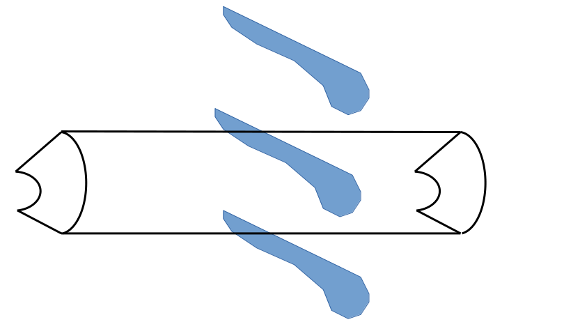
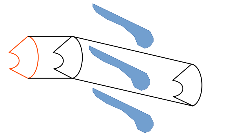
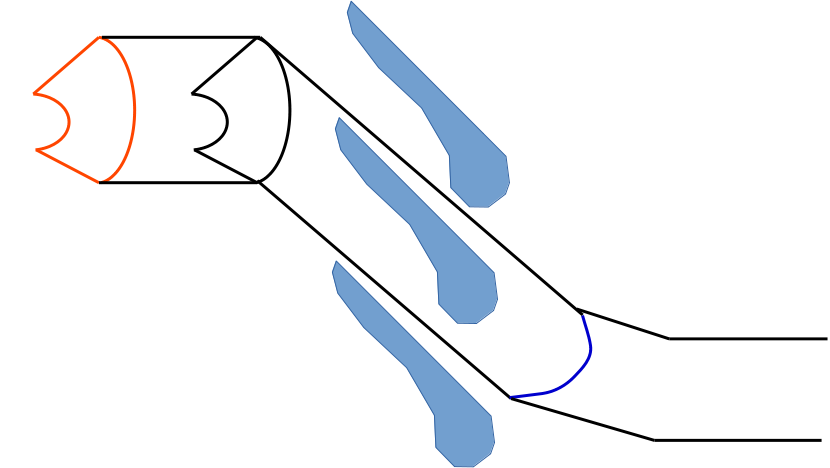
Many a times, it is a necessity to split the geometry appropriately into multiple volumes especially when this sections are present. Such splits are required to create extrudable or sweepable sections to generate either full hexahedral mesh or use thin sweeping method to generate all prism elements in narrow gaps. Splitting a body with plane is straightforward though the options to split a (solid) body with a curved plane (surface) is more frequently needed. ANSYS Discovery provides Combine operation to split solids using other solids or surfaces. In the image below where two cylinders are merged, a full cylindrical surface needs to be created (say for the vertical cylinder). This surface can be used to split the two cylinders into separate bodies.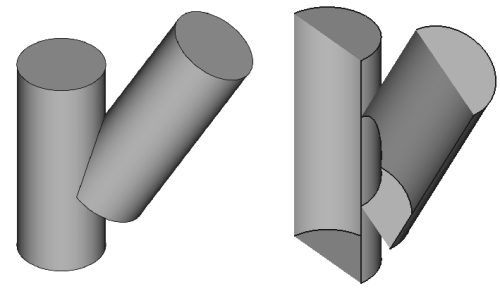
ANSYS Discovery has option to save all the components into separate files. Select the components, right-click and chose Convert to External. The icon for the component in the Structure tree changes to indicate 'external'. A batch converter converter.exe located in the install directory of Discovery can be used to convert files to other formats.
If the bodies are stored without components, directly under root components, select the bodies which needs to be saved in separate files, right click and chose "Move Each to A Component". This will move each body in separate components and the steps mentioned earlier can now be used to save them into separate files. Discovery has different type of components: internal, external, dependent and independent.
How to compare two geometry when external appearance look similar? One way is to check the surface area - the one with higher value is expected to have bigger cross-section and lengths. This can be further confirmed by comparing the volumes of the two geometries.
Data Exchange among MCAD / ECAD Tools
Navisworks (from AutoDesk) is primarily a mesh-based program, which uses polygon models to represent 3D objects. These mesh models are efficient for visualization but lack the precision and scalability of NURBS (Non-Uniform Rational B-Splines) or solids-based models used in MCAD tools. In Navisworks Simulate or Manage, export the NWD file to the FBX format. Read the FBX file in Blender and export it into STL format. Navisworks is an (intermediate) viewer and reviewer of 3D models, not to create or source of 3D models like other MCAD tools (Creo, SolidWorks, CATIA...).
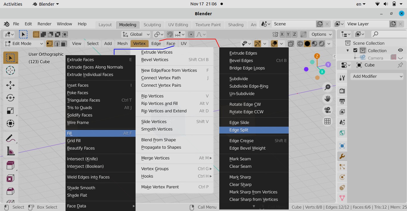
Blender Tool for Geometry Clean-up
Blender is not a CAD modelling program. For example, there is no concept of solids even if it is enclosed from all sides by faces, the concept of Boolean (add, subtract...) in Blender is not same as standard 3D CAD tools. Note that you can extrude a face and the operation is named as Solidify. Since Blender works on tessellated geometries, they are 'hollow' or "empty inside" by definition. The attributes such as mass or matter inside an object, centre of gravity... cannot be assigned to objects in Blender.Other products offering similar features are Maya 3D (AutoDesk 3d Max or 3D Studio) and Houdini. From the website of Autodesk: "What is Maya? Maya is professional 3D software for creating realistic characters and blockbuster-worthy effects. Bring believable characters to life with engaging animation tools. Shape 3D objects and scenes with intuitive modelling tools. Create realistic effects – from explosions to cloth simulation." From the official page of Houdini: "Houdini is built from the ground up to be a procedural system that empowers artists to work freely, create multiple iterations and rapidly share workflows with colleagues. In Houdini, every action is stored in a node. These nodes are then “wired” into networks which define a “recipe” that can be tweaked to refine the outcome then repeated to create similar yet unique results. The ability for nodes to be saved and to pass information, in the form of attributes, down the chain is what gives Houdini its procedural nature."
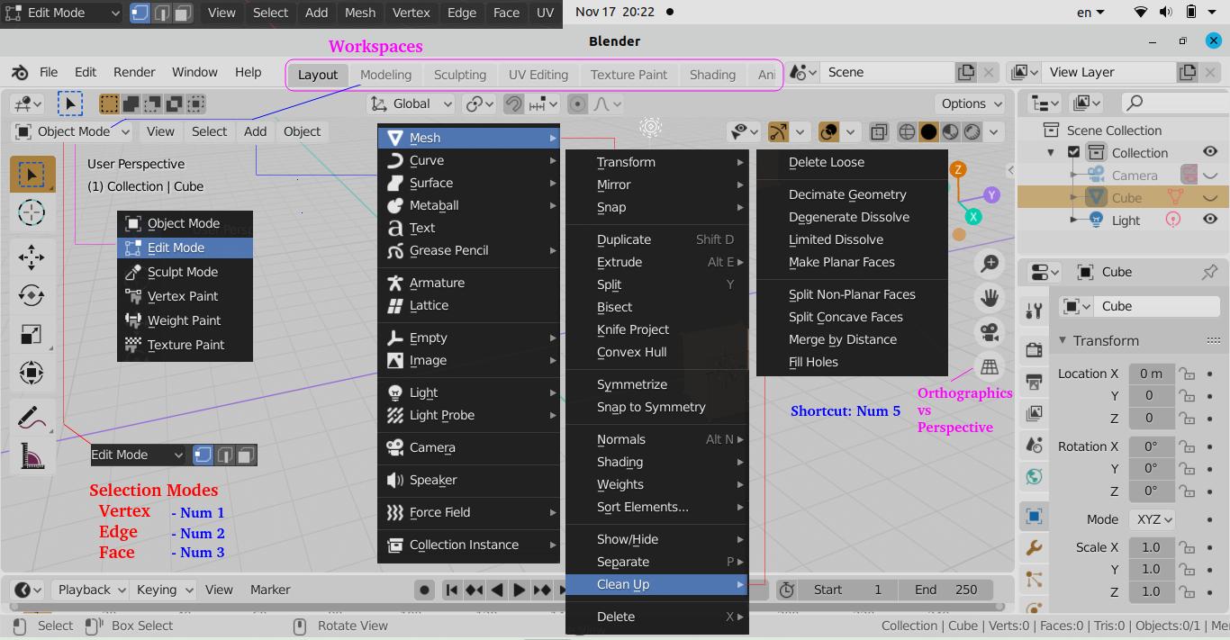
Like many feature rich applications, the interface of Blender is a bit intimidating (complex and lost in ocean type) when you open it the first time. Understaing the GUI layout and context based sub-menu is key to get started.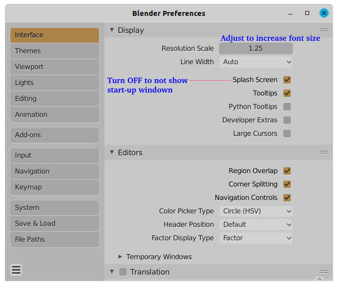
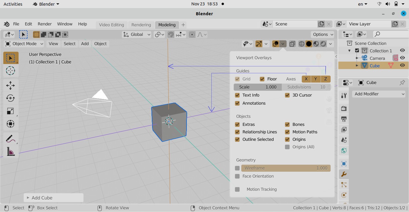
Fix for Viewport Clipping
Also known as object cut-off issue, zooming in to inspect texture or mesh details in 3D view clips faces partially like a clipping mask not showing the full model. Click on the small left arrow (< sign) on the top right near XYZ-triad to open the following pane.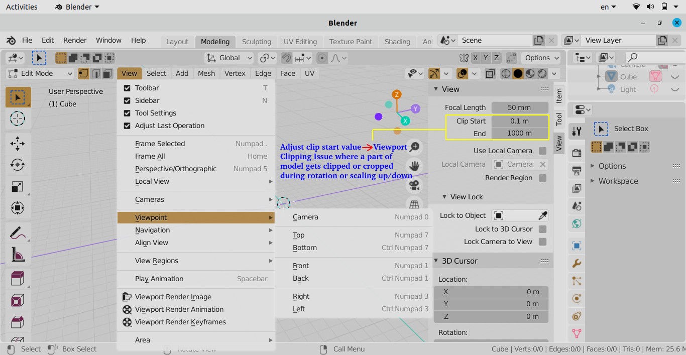
Some challenges dealing with tessellated geometries are removing fillets and chamfers from imported say STL file, deleting coincident surfaces (common boundaries of two closed volumes), removing proximities at sharp corners and point contacts such as a tire contacting flat ground.
ANSYS Discovery (known as SpaceClaim and DesignSpark) has on option called Vectorize Image that creates curves around colored areas in images. This can be used to create a 2D domain from images. A colour convention can be use to define domain and material types (solid, fluid, insulator...).
Curves
A curve or segment of a curve is defined as collection of points whose coordinates are specified as continuous ONE-parameter and single-valued mathematical functions. In Cartesian coordinate system, it can be expressed as x = f(u), y = g(u) and z = h(u) where f, g and h are the single valued mathematical functions. 'u' is known as parametric variable and it is very often (and necessarily) constrained to the interval [0 1]. The curves are said to be point-bounded as it has two definite end points.Linear parametric equation of curves: x = a + b.u, y = m + n.u, z = p + q.u where a, b, m, n, p and q are constants. The curves starts at p(u=0) = [a m p] and ends as [(a + b) (m + n) (p + q)] with direction cosines proportional to b, n and q.
Cubical parabola: x = a.u, y = b.u2, z = c.u3 where a, b and c are constants.
Left-handed circular helix: Also known as machine screw, the curves are described as x = r.cos(u), y = r.sin(u), z = p.u where r and p are constants. It is the locus (path) of a point that revolves around the z-axis at radius r and moves parallel to the z-axis at a rate proportional to the angle of revolution 'u' (known as pitch of the helix). Note that if p < 0 then it is a right-handed screw (helix).
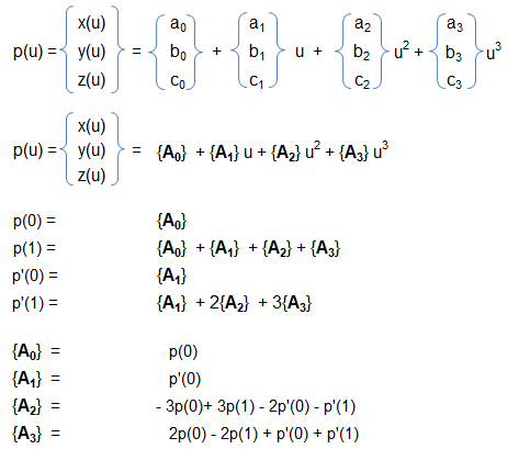
All the 3 examples above demonstrate the versatility of parametric representation of a curve. However, we need to always have a independent variable (u or θ) as parameter. Even, x or y or z themselves can be a parameter so that x=f(x), y=g(x) and z=h(x). Similarly, the surfaces can be represented parametrically. This is the reason the 3D CAD geometry in SolidWorks, Unigraphics, Creo, Inventor, FreeCAD... are called parametric models and the method is called parametric modelling.Algebraic Form of a Parametric Cubic (PC) Curve: Following 3 polynomials are required to define any curve segment of a PC curve:
x(u) = a0 + a1u + a2u2 + a3u3
y(u) = b0 + b1u + b2u2 + b3u3
z(u) = c0 + c1u + c2u2 + c3u3
The unique set of 12 constant coefficients are known as algebraic coefficients and determines the size, shape and position of the curve in space.Geometric Form of a Parametric Cubic (PC) Curve: Algebraic coefficients do not lend much flexibility to control the shape of a curve in modelling situations as they do not account for conditions as its ends points or boundaries. When a curve is described based on its conditions as the ends (such as end point coordinates, tangents, curvature, torsion...), it is called geometric form of the curve.
STEP/IGES
STEP (or STP) and IGES (or IGS) are two widely used neutral file format. IGES format was developed in 1980 by US Air Force in collaboration with Boeing, GE and Xerox. STEP format came into existence in 1984 as ISO standard 10303-21. Both these standards are plain text formats that use pre-defined special purpose syntax. For example, entity names in STEP format consists of digits preceded by '#'. /* ... */ defines comment. STEP format does not maintain features such as fillets, chamfers... as separate geometrical entities.Create Periodic Planes
The easiest option is to cut the geometry with two planes inclined at desired sector angle and passing through the axis of rotation. This option any cut through the blades (rotating as well as stationary) through the domain shall still remain periodic by definition.
Another approach is to draw a plane passing between two adjacent blades, the plane need not pass through exactly middle point of the leading edges. Create another plane inclined to the first plane at required sector angle. Split the geometry by these planes.
The following method is similar to previous one except 5 to 8 planes may be required to split the geometry into axial and tangential directions.
CAD Data Exchange
STEP format is widely used in data exchange between CAD and numerical (FEA / CFD) simulations. It has many flavours known as AP: Application Protocol. Meta data such as surface names are included when using the STEP AP214. Most of the CAD programs including Siemens NX do not include surface names in a STEP (AP 242) export by default but they do have option to make the surface names included while using AP 214 of STEP format.Similarly, to define 'names' in PTC Creo, the design can use: File > Prepare > Open Model Properties, then select 'Names' in the model properties dialogue. Then select faces by clicking > enter a name in the dialogue box opened in previous step. During CAD export to STEP format with default settings, the 'names' defined earlier do not get stored in the file. Change the export setup through File > Options > Configuration Editor > intf_out_assign_names > set it to 'user_name'.
Concept of Instance Names: In CAD assemblies, same model (or body or part) can have different instance names in different assemblies or sub-assemblies, even though it is the same model. For example, an instance name of a screw can be "bottom screw" in one assembly and "top screw" in another, even though these are the copies of same screw. CAD tools have different methods to handle instances of such geometry so that they can be identified uniquely. In Creo, the "model name" is the name of the file on disk.
Handling multiple instances of a part in assembly: this is a common requirement to use multiple copies of same parts such as nuts and bolts. However, CAD tools require unique identity for every independent part or body. This is achieved in CATIA by part name and instance name (typically a dot-integer suffix or the "Instance Name = Part Number.<Serial Number>" format). Instance names are stored within the structure of the .CATProduct file, treating them as unique identifiers for each occurrence of a component within an assembly.
CATIA, Creo, and SolidWorks use VBA / VBScript for general scripting and macro automation. Tools > Macro > Start Recording... generates a script based on user's interactive actions. File extension *.CATScript is used in Linux and *.VBScript should be used on Windows OS.
File structure in CATIA: *.CATPart file (Part Document) stores 3D geometry, including solids, surfaces, and wireframe elements retaining the full feature history. The *.CATProduct file (Assembly Document) uses a hierarchical structure to manage assemblies by referencing .CATPart files rather than embedding them. A *.CATPart has an internal "Part Number" (seen in the properties / specification tree) and an external file name (seen in Windows Explorer). While they often match, they are technically separate. CATProduct files generally use relative paths to locate their components. This means if a part file is moved or renamed outside (renaming files outside of CATIA such as in Windows File Explorer), the assembly may not open correctly and the missing part will either be ignore or must be re-linked.As per section "Naming or Renaming a product" from CATIADOC: "In a *.CATProduct, the Instance Name must be unique at one Assembly level. The Part Number must be unique within the complete assembly. By definition, the File Name is the name of the Part Number. And if you rename the Root's Part Number (and the document is not saved as a file), CATIA V5 tries to change the name of the file that is going to be saved.
Thus, "Part Number" is the unique identifier for a component within a *.CATProduct, which should typically match the "file name" for consistency of data structure. Following script can be used to rename parts in a CATIA assembly as combination of partName + _ + instanceName.Language = "VBSCRIPT"
Sub CATMain() 'The module name must be CATMain
' Get the active product document
Dim current_part As Document
Dim prt_doc As PartDocument
Set current_part = CATIA.ActiveDocument
Dim part_name as Part
Set part_name = current_part.Part
Dim body_names as Bodies
Set body_names = part_name.Bodies
Dim body_name as Body
Set body_name = Bodies.Item(1)
Dim root_name As Product
Set root_name = current_part.Product
' Call the subroutine recursively to iterate through the model-tree
RenamePartsTree root_name.Products
End Sub
Sub renamePartsTree(cad_part)
Dim i As Integer
Dim prod_name As Product
Dim part_name As String
Dim instance_name As String
Dim new_name As String
For i = 1 To cad_part.Count
Set prod_name = cad_part.Item(i)
part_name = prod_name.PartNumber
instance_name = prod_name.Name
new_name = part_name & "_" & instance_name
On Error Resume Next ' In case of naming conflicts
prod_name.Name = new_name
On Error GoTo 0
' If this is a sub-product, call recursively
If prod_name.Products.Count > 0 Then
renamePartsTree prod_name.Products
End If
Next
End Sub
In Creo, enable VB Scripting by Tools > References and then check the box for "Creo Parametric VBA API Type Library for Creo Parametric". Creo treats geometrical entities as objects. Instance Names are variations created via the Family Table (Tools > Family Table). Each instance requires a unique name (up to 31 characters), which can be edited in the table.
As per Creo user guide: "A part is a logical grouping of elements, for example, a group of elements that make up a component in a sub-assembly." Design Items is the name of the top node of the tree structure. The model tree does not list geometric entities such as surfaces, edges, and curves. There is an icon for each Model Tree item that corresponds to its object type, such as assembly, part, body or feature. For some items, a glyph near the icon shows the status of the item, for example, suppressed feature or packaged component.Displaying Reference Designators in the Model Tree: open the Tree Filters dialog box, under General Items click Annotations, click OK which will display Reference designators in the model tree. To assign or rename a reference designator in the Model Tree columns, open the Model Tree Columns dialog box. Select ECAD Params from the Type list and click ECAD_REF_DES from the list and then click on >> to move it to the Displayed list. Click OK to show reference designators in the Model Tree ECAD_REF_DES column.
Refer the article titled "About Importing ECAD Databases" on support.ptc.com to get more information.
Dim creo As Object, Dim active_model As Object, Dim gen_model As Object, Dim comp_list as Object
  Set creo = GetObject(, "Creo.Application")
  'Set active_model = creo.ActiveModel

  Set comp_list = active_model.ListComponents
  For Each comp In comp_list
    Set active_model = comp.Model
    Set gen_model = active_model.InstanceGeneric

    ' Rename if Family Table instance
    If active_model.IsInstance Then

      model_name = gen_model.Name
      instance_name = active_model.Name
      new_name = gen_model.Name & "_" & active_model.Name
      active_model.Rename new_name
    End If

  Next comp
Mapkeys are macros that record command sequences. While the resulting text file can be edited, the syntax is not officially documented by PTC and changes between versions. It does not offer programming concepts like conditionals and loops.
SOLIDWORKS: To import multiple instances of a part in STEP file separately, users must select the option to import as an assembly. This treats each instance as a unique component within that assembly. It has 3 options under Assembly Structure Mapping: [1] Default (As per the file) - keeps the assembly structure of the file and does not post-process the data, [2] Import multiple bodies as parts - creates an assembly if a multi-body part is imported in SOLIDWORKS, [3] Import assembly as multiple body part - ignores the assembly structure and creates a multi-body part if an assembly is imported in SOLIDWORKS.
Like CATIA, default behaviour of SOLIDWORKS is to assign a consecutive instance number in angle brackets <n> to each instance of a component such as Hex_Bolt<1>, Hex_Bolt<2>... To assign a alpha-numeric label to an instance, the Component Reference field in the Component Properties can be used. This component reference appears in braces {} at the end of the component name in the tree.Creo also uses two types of names: an instance name (a context name that displays in the Structure Browser) and a model name (an official model identifier).
The 3D part is the basic building block of the SOLIDWORKS mechanical design software. A SOLIDWORKS model consists of 3D solid geometry in a part or assembly document. Associativity between parts, assemblies, and drawings assures that changes made to one document or view are automatically made to all other documents and views. Features are the individual shapes that, when combined, make up the part. You can also add some types of features to assemblies. Reference geometry defines the shape or form of a surface or a solid. Reference geometry includes items such as planes, axes, coordinate systems, and points. Part documents can contain multiple solid bodies. Multibody parts are not same as assemblies. A general rule to follow is that one part (multibody or not) should represent one part number in a Bill of Materials.Features: some types of features can be added to assemblies. Surfaces are another type of feature used to create or modify solid features. Reference Geometry defines the shape or form of a surface or a solid. Reference geometry includes items such as planes, axes, coordinate systems, and points.
The document name extension for assemblies is .sldasm. Assemblies consisting of many components which can be parts or other assemblies, called sub-assemblies can be created. For most operations, the behaviour of components is the same for both types. Adding a component to an assembly creates a link between the assembly and the component. Same component can be used multiple times within an assembly. For each occurrence of the component in the assembly, the suffix <n> is incremented.
In the Component Properties dialogue box, a different value for Component Reference for each instance of a component in an assembly can be assigned. Component Reference can be used to store the reference designators for an electrical harness or printed circuit board assembly. The value appears in braces { } at the end of the component name string in the FeatureManager design tree. When different instances of the same component have different values for Component Reference, the instances can be shown as separate line items in a BOM.
FeatureManager design tree: The number of solid bodies in the part document appears in parentheses next to Solid Bodies . If several bodies are created from the same feature, an instance number appears in square brackets after each instance listed in Solid Bodies
Macros are scripts that let operations run in the SOLIDWORKS software automatically. A macro can be created and program it outside of the SOLIDWORKS software. Macros can be recorded that captures the sequence of actions and commands performed by users in the SOLIDWORKS software. Macro can be run from the Macro toolbar or the Tools menu.
CircuitWorks add-on lets users create 3D models from the file formats written by most electrical computer-aided design (ECAD) systems. Electrical and mechanical engineers can collaborate to design printed circuit boards (PCBs) that fit and function in SOLIDWORKS assemblies. CircuitWorks Lite lets all SOLIDWORKS users import IDF 2.0 and 3.0 files to create SOLIDWORKS part models.
STEP File Format
www.loc.gov: ISO 10303-21 specifies an exchange format, often known as a STEP-file, that allows product data conforming to a schema in the EXPRESS data modeling language (ISO 10303-11) to be transferred among computer systems. The content of a STEP-file is termed an "exchange structure." A schema written in EXPRESS describes a set of conditions which establishes a domain. Instances can be evaluated to determine if they are in the domain.
STEP assemblies are structured as two parallel trees. A tree of products describes the logical hierarchy of an assembly, while a tree of shapes describe the geometry of each component and its placement in space. The two trees are usually roughly parallel, with links between a product and its shape, and between corresponding product and shape relationship objects.
Geometry Parts               Geometry Topological Entities
----------------------------------------------------------
Root Part
  Assembly                   Shape Type
    Component                  Surface
      Body-x                     Edge
      Body-y                     Vertex
    Sub-Assembly             Location
      Component              Reference frame
        Body-1
        Body-2
   PRODUCT (id, name*, desc^, PRODUCT_CONTEXT id): Main or root part
     .----------------------------------'                             <-.
     |                                                                  |
   PRODUCT_CONTEXT (name - can be empty string, APPLICATION_CONTEXT id, |
     context type e.g. mechanical)                 |                    |
     .---------------------------------------------'                    |
     |                                                                  |
->APPLICATION_CONTEXT (application - can be empty string)               |
|                                                           ,-----------'
| PRODUCT_CATEGORY('part', 'NONE')                          |
| PRODUCT_RELATED_PRODUCT_CATEGORY('detail', 'desc^', (PRODUCT))
| APPLICATION PROTOCOL DEFINITION('INTERNATIONAL STANDARD','automotive_design',
|   1994, APPLICATION_CONTEXT)
`------------'

   PRODUCT_DEFINITION (name*, desc^, PRODUCT_DEFINITION_FORMATION_WITH_SPECIFIED_SOURCE,
,-- PRODUCT_DEFINITION_CONTEXT)                /|\
|                                               |
|  PRODUCT_DEFINITION_FORMATION_WITH_SPECIFIED_SOURCE (name*, 'NONE, PRODUCT, .NOT KNOWN.)
'->PRODUCT_DEFINITION_CONTEXT (name*, APPLICATION_CONTEXT, 'design')
|
|  ITEM_DEFINED_TRANSFORMATION (name*, text^, AXIS2_PLACEMENT_3D 1, AXIS2_PLACEMENT_3D 2)
|  AXIS2_PLACEMENT_3D(name*, CARTESION_POINT, DIRECTION 1, DIRECTION 2)
|                                      /|\       /|\           /|\
|  CARTESIAN_POINT (name*, (X, Y, Z))---'         |             |
|  DIRECTION (name*, (i, j, k))-------------------'-------------'
|
|  NEXT_ASSEMBLY_USAGE_OCCURRENCE(id, name*, desc^, RELATING_PRODUCT_DEFINITION
|    - parent, RELATED_PRODUCT_DEFINITION child, REFERENCE DESIGNATOR)
|        |               |
|        |               '-------------------------------------------------------.
|       \|/                                                                      |
|  RELATING_PRODUCT_DEFINITION (ID such as STEP file name, Description - may be  |
|     same as ID, formation, PRODUCT_DEFINITION_CONTEXT)                         |
|                               /|\                                              |
:--------------------------------'                                               |
|                                                                                |
|                |````````````````````````````````````````````````````````````````
|               \|/
|  RELATED_PRODUCT_DEFINITION (ID, desc^,
|     PRODUCT_DEFINITION_FORMATION_WITH_SPECIFIED_SOURCE,
'---> PRODUCT_DEFINITION_CONTEXT)

   VECTOR(", DIRECTION, MAGNITUDE)
* can be blank or empty string - string identifying the entity, DIRECTION 1 can be reference and DIRECTION 2 can be normal. The CARTESIAN POINT, DIRECTION 1 and DIRECTION 2 define the local coordinate system. REFERENCE DESIGNATOR - OPTIONAL identifier which may contain only $ symbol indicating that no further reference designator is attached to this occurrence.
^ optional
- ISO 10303-11 described the the EXPRESS schema, the language used to define abstract structures and relationships within ISO 10303
- ISO 10303-21 explains the format of a STEP file, to get the file format from the EXPRESS schema
- ISO 10303-42 contains the maths behind the definitions of points, curves, surfaces in the EXPRESS schema language.
- The header for file properties has the format FILE_NAME(name of file, time stamp*, author*, organization*, preprocessor version, originating system, authorization*). Those marked with * are usually blank. Comments can be added before or after comma between /* .... */
- steptool.com provides STEP preprocessor which is used by some commercial CAD tools such as AutoCAD Inventor
- ST-Developer V20, SwSTEP 2.0, Spatial Interop 3D are names of few STEP preprocessors.
- Lines can be split at commas to improve readability and can be enclosed in parentheses such as #123=(...); where semi-colon is the line termination character.
- STEP File Analyzer and Viewer from NIST is a free tool to generate a spreadsheet or CSV files of all entity and attribute information.
- The unique identifier start with # sign is also called 'pointer' and the keywords in capital letters are classes
- PRODUCT: One per PRODUCT_DEFINITION_FORMATION, all products (root component or parent part) in the STEP file have unique names. The RELATED_PRODUCT_DEFINITION defines a view on the component, the RELATING_PRODUCT_DEFINITION defines a view of the assembly part. Both product_definitions are definitional views.
- PRODUCT_TYPE: One per PRODUCT
- PRODUCT_RELATED_PRODUCT_CATEGORY: One per PRODUCT
- MECHANICAL_CONTEXT: One per PRODUCT
- PRODUCT_CONTEXT: One per PRODUCT
- PRODUCT_DEFINITION_CONTEXT: One per PRODUCT_DEFINITION.
- NEXT_ASSEMBLY_USAGE_OCCURRENCE (N_A_U_O): Describes the instance of component in the assembly by referring corresponding PRODUCT_DEFINITION - it is an occurrence of a component definition in the next higher parent assembly.
- N_U_A_O - gives reference designator or unique body name
- If the same component is included in the assembly several times (multiple instances), several N_A_U_O are created. The block of lines to define an instance are given below.
- ITEM_DEFINED_TRANSFORMATION - gives location vector
- PRODUCT: optional - defines component name
- PRODUCT_DEFINITION: optional
- MANIFOLD_SOLID_BREP or SHELL_BASED_SURFACE_MODEL: optional, defines surface type
- CONTEXT_DEPENDENT_SHAPE_REPRESENTATION (---, PRODUCT_DEFINITION_SHAPE): C_D_S_R describes the placement of a component in the assembly
- One CONTEXT_DEPENDENT_SHAPE_REPRESENTATION corresponds to each N_A_U_O
- SHAPE_REPRESENTATION_RELATIONSHIP_WITH_TRANSFORMATION (S_R_R_W_T): describes the location of a component in the assembly together with the C_D_S_R
- ITEM_DEFINED_TRANSFORMATION: Defines a transformation used for the location of a component in the assembly and is referred by S_R_R_W_T
- SHAPE_DEFINITION_REPRESENTATION: One per shape_representation
- PRODUCT_DEFINITION_SHAPE( 'NONE', 'NONE', PRODUCT_DEFINITION ): One per SHAPE_ DEFINITION_ REPRESENTATION and CONTEXT_ DEPENDENT_ SHAPE_ REPRESENTATION
- PRODUCT_DEFINITION: Defines a PRODUCT (a component or body or parent part), one per SHAPE_DEFINITION_REPRESENTATION
- PRODUCT_DEFINITION_FORMATION: One per PRODUCT_DEFINITION, all PRODUCT_DEFINITION_FORMATION in the STEP file have unique names
- REPRESENTATION_RELATIONSHIP defines the relationship between a part and a sub-assembly
- REPRESENTATION_RELATIONSHIP_WITH_TRANSFORMATION (R_R_W_T) defines the relative coordinate transformation between the part and the sub-assembly.
A sample geometry was created and saved in STEP format. A copy of original geometry was created and moved into another sub-assembly. The naming convention used in ANSYS Discovery was follows.
ROOT_NAME
  |
  '----COMP_1
  |     |
  |     '----BODY_1
  |
  '----COMP_2
        |
        '----BODY_2
The relation between COMP_1 and BODY_1 is established using MANIFOLD_SURFACE_SHAPE_REPRESENTATION (M_S_S_R), MANIFOLD_SOLID_BREP (M_S_B), ADVANCED_BREP_SHAPE_REPRESENTATION (A_B_S_R) and SHELL_BASED_SURFACE_MODEL (S_B_S_M). M_S_B is represented as CLOSED_SHELL(' ', (list of faces)). Faces are represented as ADVANCED_FACE(' ', (FACE_OUTER_BOUND, PLANE)). F_O_B is defined as EDGE_LOOP and PLANE is defined using AXIS2_PLACEMENT_3D. If a body or volume is not fully closed, the STEP file defines it as a SHELL or SURFACE rather than a MANIFOLD_SOLID_BREP. BREP_WITH_VOIDS (is subtype of MANIFOLD_SOLID_BREP) to represent the exterior shell and one or more internal ORIENTED_CLOSED_SHELL entities (shell normal point into the void).
Here, MANIFOLD_SOLID_BREP is the main CLASS of a single body and its lower layer is the geometric topology of the entity. A_B_S_R only records the types of parts.
#40=M_S_R_R('COMP_1', (#204), #33) - here #33 give information about units and unit conversion.
#204=S_B_S_M('BODY_1', (#203)) - here #203 is definition of bounding surfaces using OPEN_SHELL(' ', *)
The relation between ITEM_DEFINED_TRANSFORMATION (I_D_T) and COMP_1 can be established using common AXIS2_PLACEMENT_3D. Form of ITEM_DEFINED_TRANSFORMATION remains same for parts and sub-assemblies. For each component or body in the product, an individual corresponding to the class called ITEM_DEFINED_TRANSFORMATION should exist. I_D_T records the number of parts and the number of sub-assemblies, without indicating the specific types of parts and the specific reference of the assembly unit.
#35=SHAPE_REPRESENTATION('COMP_1', (#15), #33)
#49=I_D_T(' ', ' ', #48, #15)
The relation between N_A_U_O and PRODUCT can be established using P_D_W_S_S (PRODUCT_DEFINITION_WITH_SPECIFIED_SOURCE).
#219=N_A_U_O('BODY', 'BODY', 'DESC', #834, #521, $)
#521=PRODUCT_DEFINITION('COMP', 'COMP', #304, #33)
#304=P_D_W_S_S(' ', 'NONE', #509, .NOT_KNOWN.)
#509=PRODUCT('COMP' 'COMP', 'DESC', #345)
Link between N_A_U_O and actual shape (body) can also be established with following keywords
#X=PRODUCT_DEFINITION_SHAPE($, $, #1234);
#1234=N_A_U_O(...);
#2345=CONTEXT_DEPENDENT_SHAPE_REPRESENTATION(... X)
Here entry #2345 is unique and occurs only once.
In a STEP file, number of lines (n0) containing PRODUCT, PRODUCT_DEFINITION, PRODUCT_DEFINITION_CONTEXT, SHAPE_REPRESENTATION_RELATIONSHIP and SHAPE_DEFINITION_REPRESENTATION are equal. They represent total number of unique bodies or parts. The number of lines containing C_D_S_R equals the total number of instances in the STEP file (total number of components created in ANSYS Discovery).
Number of lines with C_D_S_R (n1) equals those containing ITEM_DEFINED_TRANSFORMATION. Number of lines (n2) containing (REPRESENTATION_RELATIONSHIP (... SHAPE_REPRESENTATION_RELATIONSHIP ()) is equal to (n0 + n1).
The sum of number of entries with M_S_S_R and those with A_B_S_R equals n0. Number of lines with keyword SURFACE_STYLE_USAGE is equal to lines with keyword CLOSED_SHELL which is also equal to the sum of entries with MANIFOLD_SOLID_BREP and S_B_S_M.
Based on the structure where I_D_T and N_A_U_O appear in consecutive sequences, the flow chart to find out all instances of a similar part from the STEP file would be something like this. Step-1 is to identify the PRODUCT_DEFINITION of the body. While ITEM_DEFINED_TRANSFORMATION and N_A_U_O may be used together to position components in an assembly, they do not very often occur in pairs (sequences).
① Find out all the pairs of lines containing 'FIRST' the keyword ITEM_DEFINED_TRANSFORMATION and 'NEXT' the keyword N_A_U_O. Split them first based on character '(' and then split the second item from previous split based on character ','. The last two items of line containing ITEM_DEFINED_TRANSFORMATION shall contain AXIS2_PLACEMENT_3D data (a list of origin and two axes).
② The similar split of line containing N_A_U_O shall have the names of reference designators such as C23 or R15. The fourth items shall contain PRODUCT_DEFINITION for root part or top-level assembly and and fifth items contains PRODUCT_DEFINITION about parent or component name. For deeply nested model tree, this may be complex.
③ Get the two CARTESIAN_POINTS defined in AXIS2_PLACEMENT_3D, they represent relative position of the TRANSFORMATION. The first one for parent placement and the second one is for child placement.
④ AXIS2_PLACEMENT_3D shall contain lists such as [ (0, 0, 0), (0, 0, 1), (1, 0, 0) ] and [ (50, 25, 0), (0, 0, 1), [0, 1, 0) ] - in this example the transformation is δx = 50 and δy = 25 from origin.
Note: the name of root part used for ITEM_DEFINED_TRANSFORMATION can be found using keyword PRODUCT_DEFINITION_ FORMATION_ WITH_ SPECIFIED_SOURCE.Many a time specially STEP files generated using preprocessor from steptool.com, the all the lines containing N_A_U_O are listed together. The link between Reference Designator names and their position can be established using following chain of classed.
NEXT_ASSEMBLY_USAGE_OCCURRENCE (search of this line and get name of reference designators) -▸ PRODUCT_DEFINITION_SHAPE (find the line which contains unique identifier of the this N_A_U_O) -▸ CONTEXT_DEPENDENT_SHAPE_REPRESENTATION (find the line containing this P_D_S which also contains the identifier for R_R_W_T) -▸ REPRESENTATION_RELATIONSHIP_WITH_TRANSFORMATION (last parameter contains the identifier for I_D_T) -▸ ITEM_DEFINED_TRANSFORMATION -▸ AXIS2_PLACEMENT_3D -▸ CARTESIAN_POINT and DIRECTON Above workflow was tried out on a STEP file and following sequence of lines were parsed to get the expected transformation values.Example:
#13854 = NEXT_ASSEMBLY_USAGE_OCCURRENCE ( 'NAUO2', ' ', ' ', #6280, #10242, $ );
|
'--------------------------------------------------.
\|/
#4831 = PRODUCT_DEFINITION_SHAPE ( 'NONE', 'NONE', #13854 );
|
'------------------------------------------------------.
\|/
#6316 = CONTEXT_DEPENDENT_SHAPE_REPRESENTATION ( #3332, #4831 );
|
,-----------------------------------------------'
\|/
#3332 =( REPRESENTATION_RELATIONSHIP ('NONE','NONE', #9785, #8964)
REPRESENTATION_RELATIONSHIP_WITH_TRANSFORMATION ( #7520 )
SHAPE_REPRESENTATION_RELATIONSHIP( ) ); |
,------------------------------------------------'
\|/
#7520 = ITEM_DEFINED_TRANSFORMATION ('NONE', 'NONE', #7832, #9408);
#7832 = AXIS2_PLACEMENT_3D ('NONE', #4034, #8088, #13420);
#9408 = AXIS2_PLACEMENT_3D ('NONE', #8535, #10375, #5191);
#4034 = CARTESIAN_POINT ( 'NONE', (0.0, 0.0, 19.6));
#8088 = DIRECTION ( 'NONE', (0.0, 0.0, 1.0));
#13420 = DIRECTION ( 'NONE', (1.0, 0.0, 0.0));
#8535 = CARTESIAN_POINT ( 'NONE', (0.0, 0.0, 0.0));
#10375 = DIRECTION ( 'NONE', (0.0, 0.0, 1.0));
#5191 = DIRECTION ( 'NONE', (1.0, 0.0, 0.0) ;
Surfaces are named as CYLINDRICAL_SURFACE, CONICAL_SURFACE, TOROIDAL_SURFACE, BOUNDED_SURFACE, SPHERICAL_SURFACE, B_SPLINE_SURFACE, B_SPLINE_SURFACE_WITH_KNOTS...
Closed volumes are defined by many entities named as EXTRUDED_AREA_SOLID, BOOLEAN_RESULT, EXTRUDED_FACE_SOLID, EXTRUDED_FACE_SOLID_WITH_DRAFT_ANGLE, REVOLVED_AREA_SOLID, REVOLVED_FACE_SOLID, SOLID_WITH_CIRCULAR_PATTERN...
The parsing of STEP file can be done with Open CASCADE Technology (OCCT). From opencascade.com: OCCT is an object-oriented C++ class library designed for rapid production of sophisticated domain-specific CAD/CAM/CAE applications. The C++ classes and other types are grouped into packages. Packages are organized into toolkits (libraries), to which you can link your application. Finally, toolkits are grouped into seven modules. OCCT is available as package "opencascade" in official repositories of many Linux distributions.Scripting in ANSYS Discovery / SpaceClaim
To understand the API, one needs to be familiar with the key features of an Object Oriented Programming language: class (object), methods, properties and fields. 'Component' is a class, Name is its property (accessed as comp.Name where comp is an instance of Component), GetName() is the method available for this class accessed as comp.GetName(). bb = bd.Shape.GetBoundingBox( Matrix.Identity ) - bd is an instance of Body object, GetBoundingBox() is a method, Matrix is a class and Identity is the field inside Matrix class. bb is an object of class BoundingBox with Center as one of its properties.The main prerequisite is the familiarity with SpaceClaim GUI and nomenclature. Other than the official User Guide, a short and detailed resource is the appendix in the book "Computational Fluid Dynamics: An Introduction to Modeling and Applications, 1st Edition" from McGraw Hill. The appendix on SpaceClaim can be found at "accessengineeringlibrary.com/ content/ book/... /back-matter/ appendix5". Few examples of scripts can be found at github.com/ inr-kit/ SpaceClaim_scripts. It uses IronPython which in turn uses .NET framework. The Python API is found in <ANSYS_INSTALL_DIR> v212\ scdm\ SpaceClaim .Api .V212\ API_Scripting_Class_Library.chm --Also, "discuss.ansys.com/categories/3d-design" is a good source of help and sample codes. Many of the codes on this page are either a copy or adaption of codes posted on this website.
The hierarchy of Interfaces and Classes are grouped into libraries called Namespaces. The Interface determines what attributes are available for the Object. Attributes are Properties or Functions which always returns something when called. Namespace: This is a hierarchical and structured container to organize classes, interfaces, methods, enumerated variables, and fields into logical groups, preventing naming conflicts and providing modular organization of the API functionality. The API is structured into nested namespaces, often following a hierarchy like Ansys.Discovery .Api .V[Version] .Module such as Ansys.Discovery .Api .V242 .Geometry which contains classes for modeling.
The 'Object' creation is called an Instantiation. The Functions and Properties of the Interfaces associated with that 'Class' are then available for the 'Object'. Interface: is a Class template and contains definitions for functionalities that a Class can implement. The convention used is that a 'Class' name preceded by the letter 'I' describes Interface. Interfaces are useful because of Inheritance: A Class can inherit one Class (Single Inheritance) whereas "a Class and an Interface" can inherit several Interfaces (Multi Inheritance). Enumeration is a type that consists of a set of named constants (similar to the concept of dictionaries) called the enumerator list. The 'enum' keyword is used to declare an enumeration.To use scripting, the knowledge about definitions of topological entities is critical. As per ANSYS developer portal: "The topology of a model is made of Body, Face, and Edge objects, along with other objects (shells, loops, fins, and vertices) that describe in more detail how they connect up. 1) Body inherits from ITrimmedSpace. It also provides Faces and Edges. 2) Face inherits from ITrimmedSurface. It also provides surrounding Edges. 3) Edge inherits from ITrimmedCurve. It also provides adjacent Faces.
Different terms are used: Topology objects are Body, Face, Edge, Vertex. Geometry objects are Plane, Cylinder, Line, Point. While dealing with API, one may have to decipher statements like: A DesignBody has a Shape of type Body. A DesignFace has a Shape of type Face. A DesignEdge has a Shape of type Edge.When creating new scripts through script editor (say in Python), one need to look for the 'I' prefix to identify interfaces. The autocomplete feature (drop-downs that appear after typing dot symbol) can be used to find methods (functions) and properties for those objects.
To open SpaceClaim in batch mode: "C:\Program Files\ANSYS Inc\v232\scdm\SpaceClaim.exe" /Welcome=False /Splash=False /RunScript="E:\Projects\geo_script.py" /ExitAfterScript=True /Headless=True where geo_script.py should contain IronPython script. "%awp_root241%\Discovery\Discovery.exe" --hidden -o Geo.dsco --run-script "E:\Prj\scr.py" --exit-after-script
Read a *.scdoc file using Pyhton following by running a Python script. Reference: post titled "how-to-use-code-open-scdm-scdoc-file" at discuss.ansys.com
current_dir = os.path.dirname(os.path.realpath(file))
#os.getcwd(): get the installation folder of SCDM / Discovery
#GetActiveWindow().Document.Path: get the path of currently loaded geometry
geo_file = "Project.scdoc"
scr_file = "geo_Script.py"

geo_path = os.path.join(current_dir, geo_file)
scr_path = os.path.join(current_dir, scr_file)

with open(geo_path, 'r') as scdm_file:
  geo_content = scdm_file.read()

with open(scr_path , 'r') as py_file:
  scr_content = py_file.read()
The SCDM / Discovery files are referred as Document. To open a file: File.Open(r "E:\Projects\Design-1.dsco"). To save it: DocumentHelper .GetActiveDocument() .Save(). To save as: DocumentHelper .GetActiveDocument() .SaveAs(r "E:\Projects\New.dsco")
It is important to know definitions of terms in SCDM such as 'Part', 'Body', 'Component', 'Surface'... A body with faces that form a closed (watertight) volume is considered a solid. Bodies whose faces do not 'close' fully are considered as surface bodies. Solid bodies and surface bodies can be distinguished by the icons before their names in the GUI. The Python script window in SCDM has autocomplete property of built-in variables and methods. A drop-down appears once you type the dot separator. To get properties and methods associated with a given SpaceClaim object, use Dir() command. For example, Dir(face .Edges[0] .Shape .Geometry) will give list of all properties and methods inside face .Edges[0] .Shape .Geometry.
Get the root part: part = GetRootPart(), bodyNames = GetRootPart() .GetAllBodies() or bodies = GetRootPart() .GetChildren[IDesignBody](), To get bodies with name containing a string: bodies = GetRootPart() .GetAllBodies("heat"). Get all bodies in a component: body_list = compName.GetAllBodies(). Get number of bodies in a component: n_body = body_list.Count, note that Selection.Create(bd) creates a selection of body 'bd' and does not create the 'bd'.
Get all named selections: groups = GetActiveWindow() .ActiveWindow .Groups. Such lists can be accessed by standard "for loop" in Python such as "for bd in bodyNames:" or "for ns in groupsNS:". To select all faces of a body: bd_faces = bd.Faces where bd is defined as a body earlier. To get name of a body: bd_name = bd.GetName().
Orient view in isometric direction in spaceclaim: ViewHelper.ActivateNamedView('Isometric',True). Other options for view names are ['Trimetric', 'Top', 'Bottom', 'Left', 'Right', 'Front', 'Back']
Get all components: compList = GetRootPart() .GetAllComponents(). Make a component independent (break association with instance array): makeIndep = ComponentHelper .MakeIndependent(compName, None). Get Instance Suffix of a component name: c_name = compName.Name, Get searchable name of a component: q_name = compName.GetName() - notice the parentheses. Rename a component: compName.SetName(new_name). Rename a body: bd_name.SetName( new_body_name ) - note SetName and not setName.Remove special character from body names
bodies = part.GetAllBodies()
for bd in bodies:
 if "@" in bd.Name:
   bd.SetName(bd.Name.replace("@", "_")
Multiple replacement of multiple characters, use translate function or regular expressions (regex).
Select all faces of a body
bodies = part.GetAllBodies()
face_body_1 = Selection.Create(bodies[1].Faces)
To select all bodies: select = Selection.SelectAll() or
part = Window.ActiveWindow.Document.MainPart
select = Selection.Create(part.Bodies)
Create components and activate one
comp_01 = ComponentHelper.CreateAtRoot("comp_01")
comp_02 = ComponentHelper.CreateAtRoot("comp_02")
comp_11 = ComponentHelper.CreateAtComponent(comp_01, "comp_11")
ComponentHelper.SetActive(comp_11.CreateComponents[0])
Change "Share Topology" properties of a Component:
comp = GetRootPart().Components[3]
comp.Content.ShareTopology=comp.Content.ShareTopology.Share
Get components by excluding names from a list
def selectComponentsExludeNames(exclude_names, only_root_comps=False):
  comps = []
  if (only_root_comp):
    comps = GetRootPart().Components
  else
    comps = GetRootPart().GetAllComponents()
  comp_list = []
  for comp in comps:
    if comp.GetName() not in exclude_names:
      comp_list = comp_list.append(comp)
  return comp_list
#Usage:
exclude_names = ["hsrc_fpga", "heat_sink"]
comp_list = selectComponentsExludeNames(exclude_names, True)
Set the .stl import unit system: options are Millimeters, Meters, Inches
file_stl = 'E:\surf_import.stl'
from SpaceClaim.Api.V232 import *
un = MetricUnits(MetricLengthUnit.Millimeters, MetricMassUnit.Kilograms, AngleUnit.Degrees)
importOptions = ImportOptions.Create()
importOptions.Stl.Units = un
DocumentOpen.Execute(file_stl, importOptions)
Variables can be derived through the Insert Selection (the button with the black arrow and the small green '+' symbol in the script editor). Codes related to visibility and selections: Select and invert selection --- select = Selection.GetActive() .ViewHelper .ShowAll(), result = ViewHelper.InvertVisibility().
Make faces opaque: selection = BodySelection.Create( list_of_bodies ). ColorHelper .SetFillStyle( selection, FillStyle.Default, FillStyle .Opaque).Select all faces of part, faces using index values, body and datum planes:
PartSel = Selection.Create(GetRootPart())
faces = PartSel.ConvertToFaces()
Selection.Create(GetRootPart().GetAllBodies()[0].Faces[0])
Selection.Create(GetRootPart().GetAllBodies()[0])
datumSel = Selection.Create(GetRootPart().DatumPlanes[0])
Select faces by bounding box - selects faces if they are even partially inside the bounding box: innovationspace.ansys.com/ ... /spaceclaim-script-selection-by-filterbyboundingbox
PartSel_1 = Selection.Create(GetRootPart())
Faces_1 = PartSel_1.ConvertToFaces()
PartSel_2 = Selection.Create(GetRootPart().Bodies[0])
Faces_2 = PartSel_2.ConvertToFaces()
Faces = Selection.Difference(Faces_1, Faces_2)
BBox = Box.Create(minX, minY, minZ, maxX, maxY, maxZ)
Faces_in_BB = Faces.FilterByBoundingBox(BBox)
Smart Selection
selection = PowerSelection .Faces .ByRoundRadius(Face1, PowerSelectionOptions(False), SearchCriteria .SizeComparison .SmallerOrEqual, SearchCriteria .RoundType .All)secondarySelection = Selection.Empty()
options = FillOptions()result = Fill.Execute(selection, secondarySelection, options, FillMode.ThreeD, Info1)
Codes related to body and components such as select, move, rename, add to components:
selection = Body1
result = ComponentHelper.MoveBodiesToComponent(selection, Info1)
result = RenameOject.Execute( selection, "Part_X")
selections = Body2
result = ComponentHelper .MoveBodiesToComponet(selections, Component, False, Info2).
Create named selections: w_hflux is the name of the list containing faces selected based on certain criteria.
result = NamedSelection.Create(Selection.Create( w_hflux ), Selection())
result = NamedSelection.Rename("Group1", "w_heat_flux")
primarySelection = FaceSelection.Create(GetRootPart().Bodies[1].Faces[1])
secondarySelection = Selection.Empty()
result = NamedSelection.Create(primarySelection, secondarySelection)
result = NamedSelection.Rename("Group1", "w_faces_fixed_t")
Create a named selection by using FilterByArea:
part = Selection.Create( GetRootPart())
face_list = comp.ConvertToFaces().FilterByArea(minArea, maxArea)
face_list.CreateAGroup("w_fillets")
Create named selection based on volume - note that the method GetMaster() may not appear in drop-downs generated after dot (.) is entered or may not be found in API documents. This method can also be used to select all surface bodies (volume = 0.0) and place them in a new component or layer.
def createNSbyVolume(minVolume, maxVolume):
  shapesByVol = []
  assembly = GetRootPart()
  bodies = assembly.Bodies
  for body in bodies:
    # Check for solid body and ignore surface bodies
    if (body.GetMaster().Shape.IsClosed == True):
      shape = body.Shape
      volume = shape.Volume
      if (volume >=minVolume and volume <=maxVolume):
        shapesByVol.append(body)
  return shapesByVol
Select all rounds and fillets ≤ given radius and create separate named selections for concave and convex shapes. PowerSelection method has option to filter depending on convex or concave shape. In its current form, this script searches for rounds in all available bodies.
rad = 2.5
select_convex =
  PowerSelection.Faces.ByRoundRadius(MM(rad),
  PowerSelectOptions(False, BodySelection.Create(GetRootPart().GetAllBodies())),
  SearchCriteria.SizeComparison.SmallerOrEqual,
  SearchCriteria.RoundType.Convex)
select_convex.SetActive()
result = NamedSelection.Create(select_convex, Selection.Empty())
result.CreatedNamedSelection.SetName("convex_faces")

select_concave =
  PowerSelection.Faces.ByRoundRadius(MM(float(UserRadius.Value)),
  PowerSelectOptions(False, BodySelection.Create(GetRootPart().GetAllBodies())),
  SearchCriteria.SizeComparison.SmallerOrEqual,
  SearchCriteria.RoundType.Concave)
select_concave.SetActive()
result = NamedSelection.Create(select_concave, Selection.Empty())
result.CreatedNamedSelection.SetName("concave_faces")

Selection.Clear()
Get faces aligned with specified direction and also located on the 'top' of the body in that direction.
user_direction = Direction.DirZ
//Change this to UserDirection = Direction.DirX, or any arbitrary direction
//with XYZ like Direction.Create(0.50, 0.75, 1.25)

dot_tolerance = 0.9999
top_faces = []
for body in GetRootPart().GetAllBodies():
  z_faces = []
  for face in body.Faces:
    face_normal = face.GetFaceNormal(0, 0)
    dot_product = Vector.Dot(face_normal.UnitVector, UserDirection.UnitVector)
    if dot_product > dot_tolerance:
      z_face = face.GetFacePoint(0, 0)[2]
      z_faces.append([face, z_faces])
  if len(z_faces) > 0:
    z_faces.sort(key=lambda V: V[1])
    top_faces.append(z_faces[-1][0])
Selection.Create(top_faces).SetActive()
Operation on all bodies containing a string
bodyNames = GetRootPart().GetAllBodies()
bd_names_uniq = set(bodyNames)
uniq_names_list = list(nd_names_uniq)

for bd in bodyNames:
  bd_name  = bd.GetName()
  bd_faces = bd.Faces
  # Create named selections
  ns_name = "w_" + bd_name
  Selection.Create(bd_faces).CreateAGroup(ns_name)
  if (bd_name.Contains("source")):
    ... do something ...

# Loop over faces of a body. x_cg = cg[0], y_cg=cg[1]
for face in body.Faces:
    cg = face.MidPoint().Point

ViewHelper.ShowAll()
ns_groups = Window.ActiveWindow.Groups
To create unique names of bodies in a (root) part, following code can be used.
names_list = ['Mango', 'Banana', 'Guava', 'Mango', 'Grapes', 'Mango']
def createUniqList(names_list):
  size_list = len(names_list)
  names_uniq = set(names_list)
  # Convert unique names back to a list
  uniq_list  = list(names_uniq)

  for uniq_item in uniq_list:
    n_repeat = names_list.count(uniq_item)
    i = 1
    if (n_repeat > 1):
      for itr in range(size_list):
        if (names_list[itr] == uniq_item):
          names_list[itr] = uniq_item + "_" + "{:02d}".format(i)
          i = i + 1
  return names_list
Namded Selection on Faceted Bodies
mesh_comps = GetRootPart().Meshes
dir_vector = Vector.Create(1, 0, 0)
mesh_comp_items = []
for mesh_comp in mesh_comps:
  for face in mesh_comp.Shape.Faces:
    normal = face.Normal.UnitVector
    dir_cosine = Vector.Dot(dir_vector, normal)
    if (dir_cosine >= 0.9):
      mesh_comp_items.append(mesh_comp.GetDesignMeshTopology(face))
if (len(mesh_comp_items) > 0):
  Selection.Create(mesh_comp_items).CreateAGroup("faceted_faces")
Create shapes: radSph = 100, sphBody.Create( Point.Create(MM(0), MM(0), MM(0)), Point.Create(MM(radSph), MM(radSph), MM(0)), ExtrudeType .None), x1 = 10, y1 = 25, x2 = 50, y2 = 75. Create line:
start = Point2D .Create(MM(x1), MM(y1))
end = Point2D .Create(MM(x2), MM(y2))
result = SketchLine.Create(start, end)
Get normal at given uv point of a face: normal_uv = faces[3].GetFaceNormal(0.4, 0.6)
Create point on an edge and inside a facept_edge_perc = faces[0].Edges[3].EvalProportion(0.25).Point DatumPoint.Create(GetRootPart(), "pnt_", pt_edge_perc) pt_u_v = faces[1].EvalProportion(0.25, 0.75).Point pt_u_v = faces[1].GetFacePoint[0.50, 0.25]Create lines:
line_12 = Line.CreateThroughPoints(p1, p2)
crv_nurbs = NurbsCurve.CreateThroughPoints(False, "pnt", 0.001)
crv_segment = CurveSegment.Create(crv_nurbs)
design_crv = DesignCurve.Create(GetRootPart(), crv_segment)
DatumLine.Create(GetRootPart(), "line_", line_12)
Create Cuboid from Two Diagonally Opposite Corners where dimensions are in [m]:
p1 = Point.Create(x0, y0, z0)
p2 = Point.Create(x0 + Lx, y0 + Ly, z0 + Lz)
result = BlockBody.Create(p1, p2, ExtrudeType.ForceIndependent)
Create Circular Face:
circ_normal = Direction.DirY
circ_centre = Point.Create(0, 0, 0)
circle = CircularSurface.Create(circ_rad, circ_normal, circ_centre)
Create a Torus using circle created above:
pt_origin = Point.Origin
pt_z = Direction.DirZ
rot_axis = Line.Create(pt_origin, pt_z)
x_section = Selection.Create(circle.CreateBody.Face[0])
RevolveFaces.Execute(x_section, rot_axis, DEG(360), RevolveFaceOptions())
Create Cylinder:
result = CylinderBody.Create(p1, p2, p3, ExtrudeType.ForceIndependent)
cyl_body = result.CreatedBody
or
def createCylinderBody(base_point, end_point, radius):
  direction = (end_point - base_oint).Direction.ArbitraryPerpendicular
  pt3 = end_point + (direction.UnitVector * radius)
  result = CylinderBody.Create(base_point, end_point, pt3)
Copy and Translate:
trans_vector = Vector.Create(dx, dy, dz)
result = Copy.Execute(Selection.Create(base_body))
new_body = result.CreatedObjects[0]
Move.Translate(Selection.Create(new_body), trans_vector, MoveOptions())
Extrude Face and Edge
selection = Face1
options = ExtrudeFaceOptions()
options.extrudeType = ExtrudeType.Add
result = ExtrudeFaces.Execute(selection, MM(5), options, Info1)

selection = Edge1
secondarySelection = = Axis1 #Global X-axis
options = ExtrudeEdgeOptions()
result = ExtrudeEdges.Execute(selection, secondaryselection, MM(20), options, Info2)
Create a sketch plane and point on that plane: plane = Plane.ZX, result = ViewHelper .SetSketchPlane(plane), point = Point2D .Create( MM(x1), MM(y1) ), result = SketchPoint .Create(point)
Change to Solid View mode: mode = InteractionMode .Solid, result = ViewHelper .SetViewMode(mode). Set Section View: sectionPlane = Plane .PlaneXY, result = ViewHelper .SetSectionPlane(sectionPlane). Create Datum Plane: plane = Plane.PlaneYZ, result = DatumPlaneCreater .Create(plane, False).
Create Datum Point and 1D/2D Patterns
selection = CoordinateSystem1
result = DatumPointCrestor.Create(selection, 0, 0, False, Info3)
selection = DatumPoint1
data = LinearPatterndata()

Get.PatternDinension = PatternDimensionType.Two #Remove this line for 1D pattern
data.LinearDirection = Axis1
data.CountX = 2
data.PitchX = 5
data.CountY = 3 #Remove this line for 1D pattern
data.PitchY = 8 #Remove this line for 1D pattern
result = Pattern.CreateLinear(selection, data, Info4)
Ref: innovationspace.ansys.com/ ... /discovery-spaceclaim-scripting-examples: scripts to (a) loop through bodies and its faces to identify face midpoint, compare it with center coordinates of inlet and outlet (b) create Named Selection groups – inlet, outlet, wall and fluid, by identifying the faces (inlet, outlet) based on their location.
Delete unwanted edges: SCDM/Discovery has built-in option to delete unwanted edges. However, to remove edges from specific shapes only:
sph_edges = sph_comp.GetAllBodies()[0].Edges
#sph_edges = sph_comp.GetAllBodies()[0].GetDescendants[IDesignEdge]()
edges_sph = Selection.Create(sph_edges)
Delete.Execute(edges_sph)
Codes to repair geometry and Share Topology:
result = FixInterference .FindAndFix(Info1)
result = FixSplitEdges .FindAndFix()
result = FixExtraEdges .FindAndFix(Info2)
options = FixMissingfacesOptions()
result = FixMissingFaces .FindAndFix(options, None)

result = FixImprint.FindAndFix()

options = ShareToplogyOptions()
options .Tolerance = MM(0.05)
result = ShareToplogy .FindAndFix(options, Info3)

# Create NS of the shared faces
options = ShareTopologyNamedSelectionOptions()
options.Tolerance = MM(0.10)
ShareTopologyNamedSelection.FindAndFix(options)
# Get all groups created during Share Topology operation
Connectgroups = Window.ActiveWindow.Groups
Merge Bodies: targets = BodySelection .Create(Body1), tools = BodySelection .Create(Body2), result = Combine .Merge( targets, tools ). Define material: mat_name = GetRootPart() .Bodies[0] .Material
Get Geometry Information: Get area of a face - bd_faces[0]. bd_faces[0].Shape.Perimeter, bd_faces[1].Edges.Count, By selecting edges the vertices defining the edge can be accessed. bd_faces[2].Shape.Geometry.GetType() - get type of face such as cylinder or plane. Get centroid of a face: GetRootPart( ).Bodies[1] .Faces[2] .EvalMid( ).Point.
Get face normal: GetRootPart( ).Bodies[0] .Faces[1] .GetFaceNormal(0, 0)
Get radius: face.Edges[0] .Shape .Geometry .Radius
or
face.Edges[0] .Shape .GetGeometry[Circle]() .Radius
Get mid-point: face .MidPoint() .Point
Get centre of an edge: edge.Shape .GetGeometry[Circle]() .Axis .Originvol = body .MassProperties .RawSubject or vol = body.Shape .Volume cen = vol.Center.Faces.AdjacentFaces edge = face.Shape .Edges[i] face.Shape .GetAdjacentFace(edge) Faces[i].Edges .Count Faces[i].GetTangentChain().Count
Check Common Faces
To get the common face between two bodies, all the faces have to be iterated on one body and parent(s) of each faces should be checked. If the two bodies share a face, use body[i].Faces to get the faces of a body and face[j].Bodies to get the bodies attached to faces. The face which has two bodies attached to it is the connecting face. If the two bodies do not share the same face (e.g. share topology operation should be avoided for some reason), but have two faces that are identical, loop through all the faces on each body and find the ones that have common centroids. Third option is to create named selection during Share Topology operation and loop through the faces in the NS Group. GetRootPart() .Bodies[i] .Faces[j] .Parent returns the return the Idesignbody associated with a face.
bodies = GetRootPart() .GetAllBodies()
n_if = 0
for bd in bodies:
  bd_faces, bd_names = [], []
  bd_faces = bd.Faces
  for face in bd_faces:
    bd_names.append(face.Parent.GetName())
    if len(bd_names) > 1:
      n_if = n_if + 1
print(n_if)
Match the count of number of bodies with value of variable n_if calculated above. For example, if a PCB contains 100 parts mounted on it, the value of n_if should be 100 if exactly one face of all the parts are in contact with the PCB. Another approach is to count the number of shadow or contact pairs - the value should be two times the expected number of solid-solid contacts and solid-fluid contacts.
Get the face(s) closest to a given point where coordinates are specified in millimetres and faces are searched in X-direction.
def facesClosestToPoint(p_x, p_y, p_z):
  pt = Point.Create(MM(p_x,), MM(p_x,),MM(p_x,))
  direction = Direction.DirX
  rayOrigin = pt + direction.UnitVector * (-0.001)
  face_list = RayFire.Fire(rayOrigin, direction, 1.0E-10, 1.0E-5)

  for face in face_list:
    if (isinstance(face, IDesignFace)):
      Selection.Create(face).CreateAGroup("facesClosest")
      break
Get number of total faces: numFaces = len(GetRootPart() .Bodies[0] .Faces). Get normal: norm_value = str((GetRootPart() .Bodies[0] .Faces[i] .GetFaceNormal(0, 0))). Compare normal direction of a surface with +x direction: norm_value == 'Direction: (1, 0, 0)'. Get all edges of a body: GetRootPart() .Bodies[0] .Edges, Get Z-coordinate of start point of an edge: z0 = GetRootPart() .Bodies[0] .Edges[1] .Shape .StartPoint .Z, Create a datum plane aligned to zx-plane: datumPlane = DatumPlaneCreator .Create(Point .Create(0, y0, 0), Direction.DirY) .CreatedPlanes[0]
Rotate a body about Y-axis:selection = Body1 anchor = CoordinateSystem1 axis = Move.GetAxis(anchor, HandleAxis.Y) options = MoveOptions() result = Move.Rotate(selection, axis, DEG(30), options, Info1)To access first local coordinate system: cs_loc = GetRootPart().CoordinateSystems[0], to get origin: origin_cs = cs_loc.Frame.Origin --Any other coordinate system can be refered with CoordinateSystems[i] where i = 1, 2, 3...
Get centroid of a surface of a solid body, not surface bodies. Note that instances of solid bodies are known as 'DesignBody' and instances of surface bodies are called 'IDesignBody'. Thus, IsClosed property exists in the Shape property of the DesignBody and not in the instances of IDesignBody. Method-1: mass_prop = bodies[1].MassProperties .RawSubject, cen_body_1 = mass_prop.Center. Method-2: refer the code below.
selected_items = Selection.GetActive().Items
for selected_item in selected_items:
  if not isinstance(selected_item, DesignFace):
    continue
  #if isinstance(selected_item, DesignFace):
  # or
  #is_solid = selected_item.GetMaster().Shape.IsClosed
  sel_i = Selection.Create(selected_item)
  pt = MeasureHelper.GetCentroid(sel_i)
  new_pt = SketchPoint.Create(pt)
Get mass properties: principal axes and moments about principal axes. Ref: discuss.ansys.com/ ... /how-to-get-the-combined-space-claim-mass-properties
body_list = BodySelection.Create(GetRootPart().GetAllBodies())
massProps = MeasureHelper.GetMassProperties(body_list)
mass = massProps.Mass
pa_x = massProps.PrincipleAxes.AxisX
pa_y = massProps.PrincipleAxes.AxisY
pa_z = massProps.PrincipleAxes.AxisZ
principalMomentXAxis = massProps.GetMoment(pa_x)
principalMomentYAxis = massProps.GetMoment(pa_y)
principalMomentZAxis = massProps.GetMoment(pa_z)
pa_x_dir = pa_x.Direction
pa_y-dir = pa_y.Direction
pa_z_dir = pa_z.Direction
Get centre of a body
bodyProp = GetRootPart().GetAllBodies()[0].MassProperties
bodyCenter = bodyProp.PrincipleAxes.Origin
XC = bodyCenter.X
YC = bodyCenter.Y
ZC = bodyCenter.Z
Bounding box: returns two diagonally opposite corners.
BBox = GetRootPart().GetAllBodies()[0].Shape.GetBoundingBox(Matrix.Identity)
bodyCenter = BBox.Center
xc = bodyCenter.X
yx = bodyCenter.Y
zc = bodyCenter.Z
corners = BBox.Corners
corner1 = corners[0]
corner1_X = corner1.X
One can get centroids of the faces of a body and find average to get the centroid of the body:
for face in bd.Faces:
  selection = FaceSelection.Create(face)
  centre = MeasureHelper.GetCentroid(selection)
  xc = centre.X
Get centroid of all bodies defined in Named Selection
groups = GetActiveWindow().ActiveWindow.Groups
for ns in groups:
 ns_name = ns.GetName()
 ns_members = ns.Members
 for member in ns_members:
   if (isinstance(member, DesignBody):
     mass_prop = member.MassProperties.RawSubject
     centre = mass_prop.Center
     print(centre[0], centre[1], centre[2])
Set Material Type: ref = discuss.ansys.com/ ... /how-can-i-assign-a-material-to-multiple-bodies-in-spaceclaim
mat = GetRootPart().Bodies[0].Material
matId = SpaceClaim.Api.V24.MaterialPropertyId
prop = SpaceClaim.Api.V24.MaterialProperty(matId.ElasticModulus, "Elastic Modulus", 15, None)
mat.SetProperty(prop)
mat_name = "Gray Cast Iron"
succ_local, local_mat = Window.ActiveWindow.Document.Materials.TryGetValue(mat_name)
if not succ_local:
  succ, mat = SpaceClaim.Api.V24.LibraryMaterial.Library.TryGetValue(mat_name)
  local_mat = SpaceClaim.Api.V24.DocumentMaterial.Copy(Window.ActiveWindow.Document, mat)
for body in GetRootPart().GetAllBodies():
  body.Material = local_mat
Create surface from points: SCDM has a built-in method to create list of geometry objects such as pnt_list = List[Point](), pnt_pair = List[TuplePoint, Point]](), crv_list = List[ITrimmedCurve]() or pnt_list = List(Tuple[Point, Point]](). Here .Add method is used to add items and not .Append
Ref: discuss.ansys.com/discussion/2294/create-a-surface-from-multiple-points
  from System import Tuple
  ClearAll()
  p_x = [0   5 10 20 25]
  p_y = [5  10 15 20 25]
  p_z = [10 15 20 25 30]

  n_pt = len(p_x) - 1
  points = []
  for i in range (n_pt)
    p_name = "p" + str(i)
    p_name = Point.Create(p_x[i], p_y[i], p_z[i]
    points.append(p_name)

  list_points = List[Tuple[Point, Point]](Tuple.Create(points[i-1], points[i]) for i in range(len(points)))
  list_curves = CurveSegment.Create(list_points)

  d_curves = []
  for curve in list_curves:
    curve = DesignCurve.Create(GetRootPart()
    d_curves.append(curve)

  result = Fill.Execute(Selection.Create(d_curves))
  surface = Selection.Create(result.CreatedFaces[0])
Delete.Execute(Selection.Create(d_curves))crv_list = List[ITrimmedCurve]() p1 = Point.Create(x1, y1, z1) p2 = Point.Create(x2, y2, z2) curve = CurveSegment.Create(p1, p2) crv_list.Add(curve) ... # Create surface through the curves result = PlanarBody.Create(Plane.PlaneXY, crv_list) bd = result.CreatedBody # Extrude to create a body dir = Direction.Create(0, 0, 1) face = Selection.Create(bd.Faces[0]) ExtrudeFaces.Execute(face, dir, MM(2.5), ExtrudeFaceOptions()) ViewHelper.ZoomToEntity()Alternatively: Point cloud can be imported into SpaceClaim as curves where order of coordinates in a text file is Z X Y. fit=true to fit a smooth spline through the points instead of straight line segments. polyline=false to create each curve as separate entity. A newline is required after every point data row. Go to Assembly and click on the File+ button. Select the text file formatted as described below.
3d=true
polyline=true
fit=false

Z0 X0 Y0

Z1 X1 Y1

...

Zn Xn Yn
Create washers on all bolt holes in all bodies:
hole_edges = Selection.Create(bodies).ConvertToEdges().ConvertByShape(GeometryType.Circle)
min_rad = 5.0
max_rad = 10.0
extrude_h = 2.5
for edge in hole_edges:
  if edge.Items[0].Shape.Geometry.Radius > MM(min_rad) and
    edge.Items[0].Shape.Geometry.Radius < MM(max_rad) :

    selection = edge
    direction = MoveImprintEdges.GetImprintDirection(edge, edge.ConvertToFaces()
      .ConvertByShape(GeometryType.Plane), False)
    options = MoveImprintEdgeOptions()
    result = MoveImprintEdges.Execute(selection, direction, MM(extrude_h), options)

extrude_faces = List[IDesignFace]()
list_faces = Selection. Create(GetRootPart().GetAllBodies()).ConvertToFaces()
  .ConvertByShape(GeometryType.Plane)
for face in list_faces:
  edges = face.ConvertToEdges()
  if (edges.Count == 2):
    extrude_faces.Add(face.Items[0])

Selection.Create(extrude_faces).CreateAGroup("ExtrudedFaces")
Sample Scripts from Public Domains and discuss.ansys.com
Basic Operations: Open / Save / Import - 'Window' lass refers to the graphical interaction window showing part a part or a drawing sheet.
ClearAll()
File.Open(r"E:\Sctipts\Bracket.dsco") # Open Project, Document.Open(file_name)
DocumentOpen.Execute(r"E:\Projects\Case_1.scoc", FileSettings1)
impOpt = ImportOptions.Create()
DocumentOpen.Execute(r"E:\Projects\Case_1.scoc", impOpt)

GetActiveWindow().Close               # Close currently opened window
Window.Close(GetActiveWindow())       # Close active window
# If the window being closed is the last window of the document and needs
# saving, the user will not be prompted to save changes.
DocumentHelper.CloseDocument()

# convert CAD files and save them in the same directory
import glob, os
os.chdir(r"E:\Scripts\")
for file in glob.glob("*.stp"):
  File.ResetProject()
  File.Open(os.path.join(os.getcwd(), file), ImportOptions.Create())
  File.SaveAs(os.path.join(os.getcwd(), file[:-4]+".igs"))

# Run Discovery script in batch mode
"C:\Program Files\Ansys Inc\v221\Discovery\Discovery.exe" --run-script \
"E:\Scripts\pipe.scscript" --hidden --exit-after-script
# Save Project As
File.SaveAs(r"E:\Scripts\U-Bracket.dsco")
Run Discovery script from WB project page
import os
geo_file = "E:\Scripts\pipe.scscript"
#SetScriptVersion(Version="22.1.217")
template = GetTemplate(TemplateName="Geometry")
system = template.CreateSystem()
geometry = system.GetContainer(ComponentName="Geometry")
geometry.Edit(IsDiscoveryGeometry=True)
geometry.RunScript(ScriptFile=geo_file, GeometryContainer="Geometry", useAsMacro="false")
geometry.Exit()
Create Objects and Bodies
datumPlane = DatumPlaneCreator.Create(Point.Create(0, 0, planeZ), Direction.DirZ) .CreatedPlanes[0]
def createPlaneOriginNormal(origin = [0, 0, 0], normalDirection = [0, 0, 1]):
  originPoint = Point.Create(origin[0], origin[1], origin[2])
  dirZ = Direction.Create(normalDirection[0], normalDirection[1], normalDirection[2])
  frame = Frame.Create(originPoint, dirZ)
  plane = Plane.Create(frame)
  return plane

def getGroup(groupName):
  groups = GetActiveWindow().ActiveWindow.Groups
  for group in groups:
    if group.GetName() == groupName:
      return group
  return None

def getDimensionValue(group):
  tryGetDimensionResult =  group.TryGetDimensionValue()
  if tryGetDimensionResult[0]:
    return True, tryGetDimensionResult[1]
  else:
    return False, 0

def setDimensionValue(group, value):
  group.SetDimensionValue(value)

# Fill
selection = Face1
secondarySelection = Selection.Empty()
options = FillOptions()
result = Fill.Execute(selection, secondarySelection, options, FillMode.ThreeD, Info1)

# Thicken Faces
selection = FaceSelection.Create(Face0, Face1, Face2, Face3)
options = ThickenFaceOptions()
result = ThickenFaces.Execute(selection, Direction.Create(0.707, 0, 0.707), MM(-5), options)

# Create Rounds
selection = PowerSelection.Edges.ByLength(Edge1,
    PowerSelectOptions(True), SearchCriteria.SizeComparison.Equal)
options = ConstantRoundOptions()
result = ConstantRound.Execute(selection, MM(2.5), options, Info1)

# Create a block
startPoint = Point.Create(MM(5), MM(5), MM(15))
endPoint = Point.Create(MM(20), MM(20), MM(20))
BlockBody.Create(startPoint, endPoint)

# Create rectangles
RectangularSurface.Create(MM(40), MM(5),Point.Origin)
RectangularSurface.Create(MM(5), MM(40),Point.Origin)

# Merge rectangles
allSurfaceBodies = PowerSelection.Bodies.AllSurfaceBodies()
result = Combine.Merge(allSurfaceBodies)

# Create a plane and switch to sketch mode
origin  = [MM(5), MM(5), MM(5)]
plane = create_a_plane_from_origin_and_normal(origin)
ViewHelper.SetSketchPlane(plane)

# Sketch Spline
points = List[Point2D]()
points.Add(Point2D.Create(MM(0), MM(15)))
points.Add(Point2D.Create(MM(5), MM(5)))
points.Add(Point2D.Create(MM(15), MM(0)))
result = SketchNurbs.CreateFrom2DPoints(False, points)
splineCurve = result.CreatedCurves[0]

# Switch to 3D mode
mode = InteractionMode.Solid
ViewHelper.SetViewMode(mode)

# Extrude spline
selection = Selection.Create(splineCurve)
options = ExtrudeEdgeOptions()
result = ExtrudeEdges.Execute(selection, Point.Origin, Direction.DirZ, MM(30), options)
resultFace = result.CreatedFaces

## Slice block by resultFace
toolFaces = Selection.Create(resultFace)
selection = PowerSelection.Bodies.AllSolidBodies()
result = SplitBody.ByCutter(selection, toolFaces, True)

sel_body  = Selection.Create(GetRootPart().Bodies[0])
sel_datum = Selection.Create(datum_plane)
SplitBody.Execute(sel_body, sel_datum)

# delete unncessary bodies
referencePoint = Point.Create(MM(5), MM(5), MM(15))
for body in GetRootPart().GetAllBodies():
  if not body.Shape.ContainsPoint(referencePoint):
    body.Delete()

# Extrude resulting surface body
faceToExtrude = result.GetModified[IDesignFace]()
faceToExtrudeSelection = Selection.Create(faceToExtrude)
options = ExtrudeFaceOptions()
options.ExtrudeType = ExtrudeType.Add
result = ExtrudeFaces.Execute(faceToExtrudeSelection, MM(40), options)

# Create the named selections
Selection.Create(GetRootPart().Bodies).CreateAGroup("SolidBody")
for face in GetRootPart().Bodies[0].Faces:
  if (face.Shape.ContainsPoint(Point.Create(MM(2.5), 0, MM(2.5)))):
    Selection.Create(face).CreateAGroup("Fixed support")
  if (face.Shape.ContainsPoint(Point.Create(0, MM(2.5), MM(2.5)))):
    Selection.Create(face).CreateAGroup("Pressure load")

#How to Access Groups
groups = GetActiveWindow().ActiveWindow.Groups
for group in groups:
  print group.GetName()

#How to get all items of a Group/Named Selection
group = GetActiveWindow().ActiveWindow.Groups[0]
Group.Members
#or
Selection.CreateByGroups("Height").Items
heightGroup = getGroup("Height")

tryGetDimensionResult =  heightGroup.TryGetDimensionValue()
print(tryGetDimensionResult)
Get and Set Dimension Values
for group in groups:
  if not group.HasDimension:
    group.Delete()

topGroup = getGroup("Top")
tryGetDimensionResult =  topGroup.TryGetDimensionValue()
print(tryGetDimensionResult)

heightGroup = getGroup("Height")
success, height = getDimensionValue(heightGroup)
if success:
  print(height)

heightGroup.SetDimensionValue(MM(5))
if success:
  print(height)
  setDimensionValue(heightGroup, height + MM(4))
Using script parameter to create a surface
Test = Parameters.Test
RectangularSurface.Create(Test, Test, Point.Origin)

#Units of Script Parameters
Length = Parameters.Length
myUnits = UnitsHelper.GetDocumentUnits()
print("Parameter - SI units: " + str(Parameters.Length))
print("Parameter - local units (" + myUnits.LengthProperties.Type.ToString() \
  + "): " + str(Parameters.Length*myUnits.LengthFactor))

#Set radius2 to initial value minus radius1 divided by 3
r1Group = getGroup("radius1")
success, radius1 =  getDimensionValue(r1Group)
r2Group = getGroup("radius2")
success, radius2 =  getDimensionValue(r2Group)
if success:
  print(radius2)
  setDimensionValue(r2Group, radius2 - radius1/3)
Objects, Selections and Named Selections
#Access Bodies: select bodies using part.Bodies
Selection.Clear()
part = GetRootPart()
bodies = part.Bodies
selection = Selection.Create(bodies)
selection.SetActive()

#Access Bodies: select bodies using part.GetBodies()
part = GetRootPart()
bodies = part.GetBodies()
selection = Selection.Create(bodies)

#select bodies using part.GetBodies(“filter”)
part = GetRootPart()
bodies = part.GetBodies("_2")
selection = Selection.Create(bodies)

#listing bodies using part.GetAllBodies()
part = GetRootPart()
bodies = part.GetAllBodies()
for body in bodies:
  print(body.GetName())

#Index of bodies
part = GetRootPart()
bodies = part.GetAllBodies()
for index,body in enumerate(bodies):
    print(index,body.GetName())

# Access Components:
part = GetRootPart()
for component in part.Components:
  print(component.GetName())

part = GetRootPart()
for component in part.GetAllComponents():
  print(component.GetName())

# Access Coordinate System:
part = GetRootPart()
for coordinateSystem in part.CoordinateSystems:
  print(coordinateSystem.GetName())

for coordinateSystem in part.Components[0].GetCoordinateSystems():
  print(coordinateSystem.GetName())

for coordinateSystem in part.Components[0].GetAllCoordinateSystems():
  print(coordinateSystem.GetName())

for coordinateSystem in part.GetDescendants[ICoordinateSystem]():
  print(coordinateSystem.GetName())

# Access Datum Plane
part.DatumPlanes
part.Components[0].GetDatumPlanes()
part.Components[0].GetAllDatumPlanes()

# Access Datum Lines
part.DatumLines
part.Components[0].GetDatumLines()
part.Components[0].GetAllDatumLines()

# Access Datum Points
part.DatumPoints
part.Components[0].GetDatumPoints()
part.Components[0].GetAllDatumPoints()
Setting colour of faces
Colour names can be defined in a list: clr_list = [ColorHelper.Magenta, ColorHelper.Blue, ColorHelper.Cyan, ColorHelper.Red, ColorHelper.Azure]# Getting Faces of body:
bd_list = GetRootPart().Bodies[0]
for face_i in bd_list.Faces:
geo_type = face_i.Shape.Geometry
if isinstance(geo_type, Cone):
ColorHelper.SetColor(Selection.Create(face_i), ColorHelper.Azure)
if isinstance(geo_type, Plane):
ColorHelper.SetColor(Selection.Create(face_i), ColorHelper.Olive)
if isinstance(geo_type, Cylinder):
ColorHelper.SetColor(Selection.Create(face_i), ColorHelper.Violet)
selection = BodySelection.Create(GetRootPart().Components[0].Content.Body[0]))
options = SetColorOptions()
options.UseAlpha = True
options.Exact = True
options.RandomColor = False
options.RandomSeed = 0
options.EdgeColorTarget = EdgeColorTarget.Body
options.FaceColorTarget = FaceColorTarget.Body
ColorHelper.SetColor(selection, options, Color.FromArgb(255, 255, 0, 128))
# Change colour of surfaces
i=0
for body in GetRootPart().GetAllBodies():
if body.Master.Shape.IsClosed==False:
thick=body.GetMidSurfaceAspect().GetThickness()
if thickness.has_key(thick)==False:
thickness[thick] = clr_list[i]
i = i + 1
ColorHelper.SetColor(Selection.Create(body), SetColorOptions(), thickness.get(thick))
# Change colour of parts of type Beam
from SpaceClaim.Api.V212 import PartType
i=0
for item in GetRootPart().Components:
part = item.Content.GetMaster()
if part.Type == PartType.BeamProfile:
beam_profiles[part]=color[i]
i = i + 1
for beam in GetRootPart().GetDescendants[IBeam]():
'''
sect = beam.GetMaster().SectionSource
if beam_profiles.has_key(sect)==False:
beam_profiles[sect]=color[i]
i = i + 1
'''
ColorHelper.SetColor(Selection.Create(beam), SetColorOptions(),
beam_profiles.get(beam.GetMaster().SectionSource))
# Getting Descendants
bd_list = GetRootPart().Bodies[0]
edge_list = bd_list.GetDescendants[IDesignEdge]() #IBeam
selection = Selection.Create(edge_list)
selection.SetActive()
# Getting newly created entities:
bd_list = GetRootPart().Bodies[0]
edge_list = bd_list.GetDescendants[IDesignEdge]()
selection = Selection.Create(edge_list)
options = ConstantRoundOptions()
result = ConstantRound.Execute(mySel, MM(1), options)
selection = Selection.Create(result.CreatedFaces)
ColorHelper.SetColor(mySelection, ColorHelper.Cyan)
cfaces = result.CreatedFaces
length_cfaces = len(cfaces)
# Getting Modified entities
bd_list = GetRootPart().Bodies[0]
edge_list = bd_list.GetDescendants[IDesignEdge]()
sel = Selection.Create(edge_list)
options = ConstantRoundOptions()
result = ConstantRound.Execute(sel, MM(1), options)
selection = Selection.Create(result.CreatedFaces)
ColorHelper.SetColor(selection, ColorHelper.Cyan)
selection = Selection.Create(result.GetModified[IDesignFace]())
ColorHelper.SetColor(selection, ColorHelper.Magenta)
# Operating on Object lists
body_list = GetRootPart().GetAllBodies()
Selection.Create(body_list).SetActive()
body_list.Remove(GetRootPart().GetAllBodies()[1])
Selection.Create(body_list).SetActive()
body_list.Remove(GetRootPart().GetAllBodies()[2])
Selection.Create(body_list).SetActive()
body_list.Add(GetRootPart().GetAllBodies()[1])
Selection.Create(body_list).SetActive()
Selecting entities using Power Selection
sel_0 = Selection.GetActive()
for body in sel_0.GetItems[IDesignBody]():
  print(body.GetName())
sel_1 = Selection.CreateByNames("Cylinder")
sel_1.SetActive()
Selection.Clear()
sel_1.GetInverse().SetActive()

sel_2 = Selection.CreateByGroups("Top")
sel_2.SetActive()

sel_3 = Selection.CreateByNames("Box")
sel_3.AddToActive()

sel_4 = Selection.SelectAll()
sel_4.SetActive()

sel_5 = mySel_4 - mySel_3
sel_5.SetActive()

# gets the current selection from the active view
sel_6 = Selection.GetActive()

# create inverted selection
sel_7 = mySel_1.GetInverse()

# select objects from this selection in active view
sel_8.SetActive()

# Power Selection
seedSelection = Selection.CreateByNames("b07")
powSelection = PowerSelection.Bodies.ByVolume(seedSelection,
PowerSelectOptions(True),
SearchCriteria.SizeComparison.SmallerOrEqual)
powSelection.SetActive()

seedSelection = Selection.CreateByNames("b08")
powSelection = PowerSelection.Bodies.ByVolume(seedSelection,
PowerSelectOptions(False),
SearchCriteria.SizeComparison.SmallerOrEqual)
powSelection.SetActive()

# Power Selection – selecting other bodies
otherBodies=Selection.Create(GetRootPart().GetAllBodies())
options=PowerSelectOptions(False, otherBodies)
seed=Selection.Create(GetRootPart().GetAllBodies("b03"))
pSel=PowerSelection.Bodies.ByVolume(seed, options, \
  SearchCriteria.SizeComparison.LargerOrEqual)
pSel.SetActive()

otherBodies=Selection.Create(GetRootPart().GetBodies())
options=PowerSelectOptions(False, otherBodies)
seed=Selection.Create(GetRootPart().GetAllBodies("b04"))
pSel=PowerSelection.Bodies.ByVolume(seed, options, \
  SearchCriteria.SizeComparison.LargerOrEqual)
pSel.SetActive()

# Power Selection – selecting seed
options=PowerSelectOptions(True,None,True)
seed=Selection.Create(GetRootPart().GetAllBodies("b07"))
pSel=PowerSelection.Bodies.ByVolume(seed, options, \
  SearchCriteria.SizeComparison.SmallerOrEqual)
pSel.SetActive()

options=PowerSelectOptions(True,None,False)
seed=Selection.Create(GetRootPart().GetAllBodies("b07"))
pSel=PowerSelection.Bodies.ByVolume(seed, options, \
  SearchCriteria.SizeComparison.SmallerOrEqual)
pSel.SetActive()

# Multiple Objects Selection
b1 = GetRootPart().Bodies[0]
b2 = GetRootPart().Bodies[1]
b3 = GetRootPart().Bodies[2]
# Approach 1
s1 = Selection.Create(b1, b2, b3)
# Approach 2
body_list = [b1, b2]
body_list.Add(b3)
s2 = Selection.Create(body_list)
# Approach 3
list = List[IDesignBody]()
list.Add(b1)
list.Add(b2)
list.Add(b3)
s3 = Selection.Create(list)
# Approach 4
s4 = Selection.Create(b1, b2)
s4 = s4 + Selection.Create(b3)
s4.SetActive()

# Mixed Selections
b1 = GetRootPart().Bodies[0]
b2 = GetRootPart().Bodies[1]
b3 = GetRootPart().Bodies[2]
f1 = b3.Faces[0]
f2 = b3.Faces[1]
# Approach 1
s1 = Selection.Create(b1, b2, f1, f2)
# Approach 2
b_list = [b1, b2]
f_list = [f1, f2]
s2 = Selection.Create(b_list + f_list)
s2.SetActive()

# Multiple objects selection
b1 = GetRootPart().Bodies[0]
b2 = GetRootPart().Bodies[1]
b3 = GetRootPart().Bodies[2]
f1 = b3.Faces[0]
f2 = b3.Faces[1]
b_list = [b1, b2]
f_list = [f1, f2]
sel1 = Selection.CreateByObjects([b1, f_list])
sel2 = Selection.CreateByObjects([b_list, f_list])
sel3 = Selection.Create(b1, f1, f2)
sel3.SetActive()
Create Named Selections
for face in GetRootPart().Bodies[0].Faces:
  ns = NamedSelection.Create(Selection.Create(face), Selection())
  if isinstance(face.Shape.Geometry, Cylinder):
    ns.CreatedNamedSelection.SetName("sideWall")
  elif face not in Selection.CreateByGroups("inlet").GetItems[IDesignFace]():
    ns.CreatedNamedSelection.SetName("outlet")
  else:
    ns.CreatedNamedSelection.Delete()

ns = NamedSelection.Create(Selection.CreateByNames("cylinder"), Selection())
nsName = ns.CreatedNamedSelection.GetName()
NamedSelection.Rename(nsName, "cylinder_faces")
Selection.Create(GetRootPart().Bodies[0]).CreateAGroup("cyl_faces")

part = GetRootPart()
for component in part.Components:
  bodies = component.GetAllBodies()
  selection = Selection.Create(bodies)
  selection.SetActive()
  # Move bodies to root component
  result = ComponentHelper.MoveBodiesToComponent(selection, part, False)

# Delete Empty Components
ComponentHelper.DeleteEmptyComponents(part)

Selection.Clear()
body_list = List[IDesignBody]()
part = GetRootPart()
for body in part.GetAllBodies():
  if body.Shape.Volume <= 3e-07 :
    body_list.Add(body)
Selection.Create(body_list).SetActive()

tolerance = 3e-7
for body in GetRootPart().GetAllBodies():
  if body not in GetRootPart().GetBodies():
    ComponentHelper.MoveBodiesToComponent(Selection.Create(body),\
    GetRootPart().Root)

for comp in GetRootPart().GetAllComponents():
  ComponentHelper.DeleteEmptyComponents(Selection.Create(comp))

powerSel = PowerSelection.Bodies.ByVolume(tolerance, None, \
 SearchCriteria.SizeComparison.SmallerOrEqual)
powerSelInv = Selection.Create(GetRootPart().GetAllBodies())-powerSel
result = ComponentHelper.MoveBodiesToComponent(powerSel)
result.CreatedComponents[0].SetName("smallBodies")
result = ComponentHelper.MoveBodiesToComponent(powerSelInv)
result.CreatedComponents[0].SetName("bigBodies")
Creating cylinders by extruding surfaces
ClearAll()
Diameter = [10, 30, 20, 40, 60]
Length   = [50, 75, 25, 10, 60]
z_offset = 100
# cylinder creation version 1
for i in range(len(Diameter)):
  face_i = CircularSurface.Create(Diameter[i]/2,
    Direction.DirZ,
    Point.Create(0, 0,
      sum(Length[:i])-Length[0] + z_offset)).CreatedBody.Faces
  options = ExtrudeFaceOptions()
  options.ExtrudeType = ExtrudeType.ForceIndependent
  result = ExtrudeFaces.Execute(Selection.Create(face_i), Length[i], options)
  result.CreatedBodies[0].SetName("Cylinder_v1_"+str(i))
Selection.Clear()
ViewHelper.ZoomToEntity()

# Solidify Sketch
mode = InteractionMode.Solid
result = ViewHelper.SetViewMode(mode)

# Demo 2
# cylinder creation version 2
for i in range(len(Diameter)):
  CenterBottom=Point.Create(0, (sum(Length[:i]) - Length[0]) + z_offset, 0)
  CenterTop=Point.Create(CenterBottom.X,
                           CenterBottom.Y + Length[i], CenterBottom.Z)
  DragPoint=Point.Create(Diameter[i]/2.,
      CenterTop.Y, CenterTop.Z)
  result=CylinderBody.Create(CenterBottom,
                             CenterTop, DragPoint, ExtrudeType.ForceIndependent)
  result.CreatedBodies[0].SetName("Cylinder_v2_"+str(i))
Selection.Clear()
ViewHelper.ZoomToEntity()

# Solidify Sketch
mode = InteractionMode.Solid
result = ViewHelper.SetViewMode(mode)

#Demo 3
ClearAll()
from math import tan, pi
ConeHeight=0.02
ConeAngle=DEG(30)

ViewHelper.SetSketchPlane(Plane.PlaneXY)

pt1 = Point2D.Create(0, 0)
pt2 = Point2D.Create(0, ConeHeight)
pt3 = Point2D.Create(ConeHeight*tan(ConeAngle/2), 0)

SketchLine.Create(pt1, pt2)
SketchLine.Create(pt2, pt3)
SketchLine.Create(pt3, pt1)

result=ViewHelper.SetViewMode(InteractionMode.Solid)

sel = Selection.Create(result.CreatedBodies[0].Faces)
axis = Line.Create(Point.Origin,Direction.DirY)
options = RevolveFaceOptions()
options.ExtrudeType = ExtrudeType.Add
RevolveFaces.Execute(sel, axis, DEG(360), options)

Selection.Clear()
ViewHelper.ZoomToEntity()

# Demo 4
ClearAll()
pt1=Point.Origin
pt2=Point.Create(MM(10), MM(2), MM(2))

result=BlockBody.Create(pt1, pt2, ExtrudeType.Add)
b0=result.CreatedBody
for i in range(10):
  sel = Selection.Create(b0)
  direction = Direction.DirY
  options = MoveOptions()
  options.Copy = True
  result = Move.Translate(sel, direction, (i+1)*MM(10), options)
Selection.Clear()
ViewHelper.ZoomToEntity()

# Demo 5
ClearAll()
pt1=Point.Create(MM(-10),MM(0),MM(0))
pt2=Point.Create(pt1.X+MM(2), pt1.Y+MM(2), pt1.Z+MM(2))

result=BlockBody.Create(pt1, pt2, ExtrudeType.Add)
b0=result.CreatedBody
for i in range(11):
    mySel = Selection.Create(b0)
    axis = Line.Create(Point.Origin, Direction.DirZ)
    options = MoveOptions()
    options.Copy = True
    result = Move.Rotate(mySel, axis, (i+1)*DEG(30), options)
Selection.Clear()
ViewHelper.ZoomToEntity()

# Demo
from SpaceClaim.Api.V21 import Command
import os
ClearAll()
#Import the geometry
doc_path = os.path.dirname(GetActiveWindow().Document.Path)
DocumentInsert.Execute(os.path.join(doc_path, "valve1.dsco"))
Selection.Create(GetRootPart().Components[0]).SetActive()
c = Command.GetCommand("ImportComponentGroups")
c.Execute()
ViewHelper.ZoomToEntity()

#Fill the surface holes < criteria
criteria_radius = MM(7)
total_selection = Selection.Empty()
selection1 = PowerSelection.Faces.BySurfaceHoleRadius(criteria_radius,
    PowerSelectOptions(True),
    SearchCriteria.SizeComparison.SmallerOrEqual)
total_selection += selection1
total_selection.SetActive()
result = Fill.Execute(total_selection)
Remove all chamfers and rounds
criteria_radius = MM(2)
total_selection = PowerSelection.Faces.ByRoundRadius(criteria_radius,
    PowerSelectOptions(True),
    SearchCriteria.SizeComparison.SmallerOrEqual,
    SearchCriteria.RoundType.All)
for body in GetRootPart().GetAllBodies():
  for face in body.Faces:
    if isinstance(face.Shape.Geometry, Cone):
      total_selection += Selection.Create(face)
total_selection.SetActive()
result = Fill.Execute(total_selection)

#Create missing bodies from Named Selections and move them to new components
ComponentHelper.SetActive(Selection.Create(GetRootPart().Components[0]), None)
options = LoftOptions()
options.IsRuled = True

selection = Selection.CreateByGroups("inlet_1")
selection += Selection.CreateByGroups("inlet_2")
result = Loft.Create(selection, None, options)
selection = Selection.Create(result.CreatedBodies[0])
result = ComponentHelper.MoveBodiesToComponent(selection)
result.CreatedComponents[0].SetName("inlets")

#Simplify 1 body
body = GetActivePart().GetAllComponents("Valve")[0].GetBodies()[0]
zmax = 0
for face in body.Faces:
  if face.EvalMid().Point.Z > zmax:
    zmax = face.EvalMid().Point.Z
    my_face = face
selection = Selection.Create(my_face) +  Selection.Create(my_face.AdjacentFaces)
result = Fill.Execute(selection)
Remove / Translate / Copy Holes
sel = PowerSelection.Faces.BySurfaceHoleRadius(MM(3),
       PowerSelectOptions(False, BodySelection.Create(GetRootPart().Bodies[0])),
       SearchCriteria.SizeComparison.Equal)
secondarySelection = Selection.Empty()
options = FillOptions()
result = Fill.Execute(sel, secondarySelection, options, FillMode.ThreeD)

# Translate bigger hole Along X Handle
circ_face = PowerSelection.Faces.BySurfaceHoleRadius(MM(35),
       PowerSelectOptions(False, BodySelection.Create(GetRootPart().Bodies[0])),
       SearchCriteria.SizeComparison.Equal)
direction = Direction.Create(1, 0, 0)
options = MoveOptions()
result = Move.Translate(circ_face, direction, MM(45), options)

# Translate (copy) bigger hole Along X Handle
direction = Direction.Create(1, 0, 0)
options = MoveOptions()
options.CreatePatterns = True
options.Copy = True
result = Move.Translate(circ_face, direction, MM(-90), options)
Create Fluid Volume
part = GetRootPart()
body = part.Bodies[0]
ymin = 0
ymax = 0
zmax = 0
# access faces with openings (ymin, ymax, zmax)
for face in body.Faces:
  if face.EvalMid().Point.Y < ymin:
    ymin = face.EvalMid().Point.Y
    ymin_face = face
  if face.EvalMid().Point.Y > ymax:
    ymax = face.EvalMid().Point.Y
    ymax_face = face
  if face.EvalMid().Point.Z > zmax:
    zmax = face.EvalMid().Point.Z
    zmax_face = face
options = VolumeExtractOptions()
selection = FaceSelection.Create(ymin_face, ymax_face, zmax_face)
#select seed face
secondarySelection = circ_face
result = VolumeExtract.Create(selection, secondarySelection, options)
External Connections such as MS-Excel
#Reference to Microsoft Excel
ClearAll()
clr.AddReference("Microsoft.Office.Interop.Excel")
import Microsoft.Office.Interop.Excel as Excel
import os

doc_path = os.path.dirname(GetActiveWindow().Document.Path)
doc_excel = Excel.ApplicationClass()
doc_excel.Visible = True
excel_file_name = "read_excel.xlsx"
wb = doc_excel.Workbooks.Open(os.path.join(doc_path,excel_file_name))
#or ws = workbook.Worksheets("Sheet1")
ws = wb.Worksheets[1]
#Read data from Excel file
i = 1
myX = ""
wloc = True
points = List[Point2D]()
while wloc:
  myX = ws.Rows[i].Value2[0, 0]
  if not isinstance(myX, str):
    myY = ws.Rows[i].Value2[0, 1]
    points.Add(Point2D.Create(MM(myX), MM(myY)))
  i = i+1
  if myX == "End":
    wloc = False
wb.Close()
doc_excel.Quit()

#create spline curve from imported point data and create a surface body
ViewHelper.SetSketchPlane(Plane.PlaneXY)
result = SketchNurbs.CreateFrom2DPoints(True, points)
ViewHelper.SetViewMode(InteractionMode.Solid)
ViewHelper.ZoomToEntity()
Scripting in ANSYS DesignModeler
The script file is written in JScript (extension *.js). // Two slashes indicate a comment. Access to the DesignModeler application functions is accessible via the prefix 'agb.', as in the command: agb.Regen(); //Run 'Generate' command. Create a Boolean operation:var bool_addBodies= ag.gui .CreateBoolean();
bool_addBodies.Name = "Add Bodies";
bool_addBodies.Operation = 0;
ag.listview .ActivateItem("Tool Bodies");
agb.ClearSelections();
body_1 = ag.fm.Body(1);
agb.AddSelect(agc.TypeBody, body_1);
body_2 = ag.fm.Body(2);
agb.AddSelect(agc.TypeBody, body_2);
ag.listview .ItemValue = "Apply";
Script Constants: These must be prefixed with agc to be usable such as agc.Add //Add Material. FormNewPartFromAllBodies(); FormNewPartFromSelectedBodies(); Properties: 'Name' allows the part to be named; for example, px.Name = "Origin_x";
Scripting in Cadence's Fidelity Pointwise
The scripting language is known as Glyphs which is implemented as a set of Tcl/Tk (Tool command Language / Tool kit) procedures. Pointwise supports non-Tcl scripting (or binary code) applications through a feature called Glyph Server.Geometry Editing in FreeCAD
FreeCAD works using module or workbench defined in the drop-down shown below. Hover the mouse near the bottom right corner shown below to select the Navigation Style and associated mouse key mapping.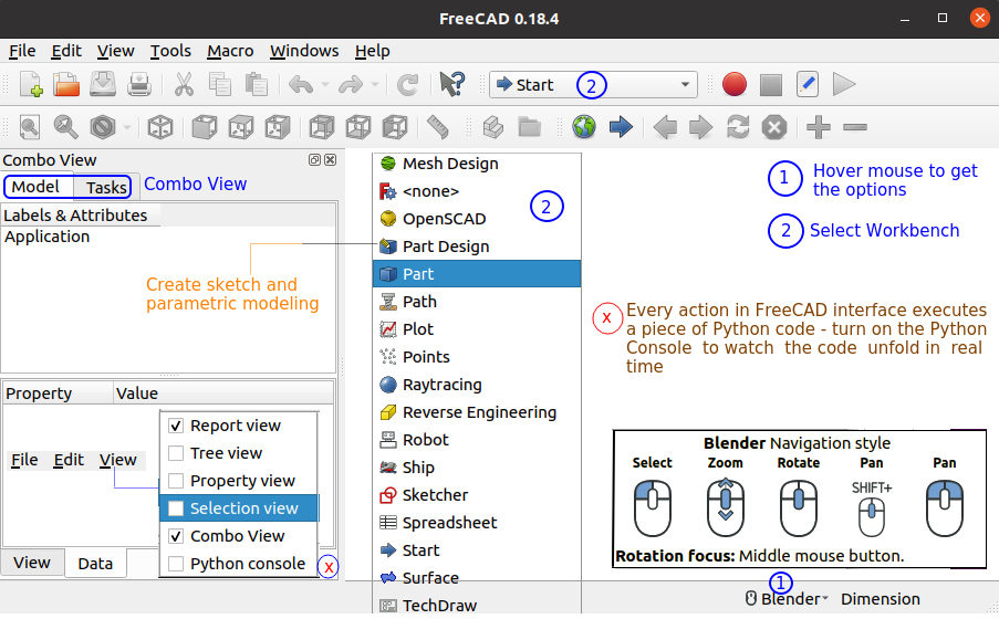
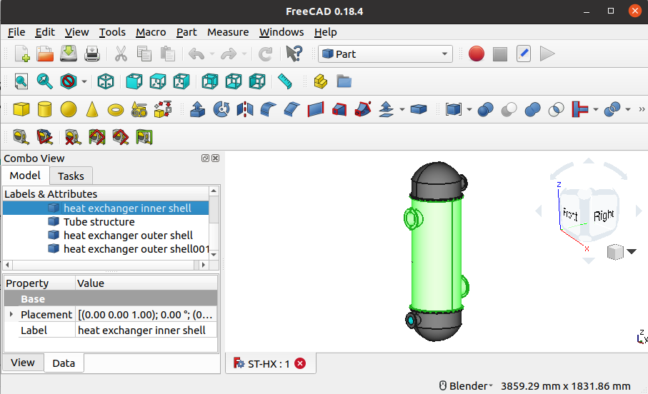
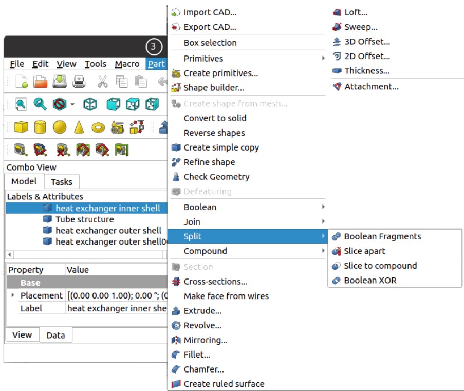
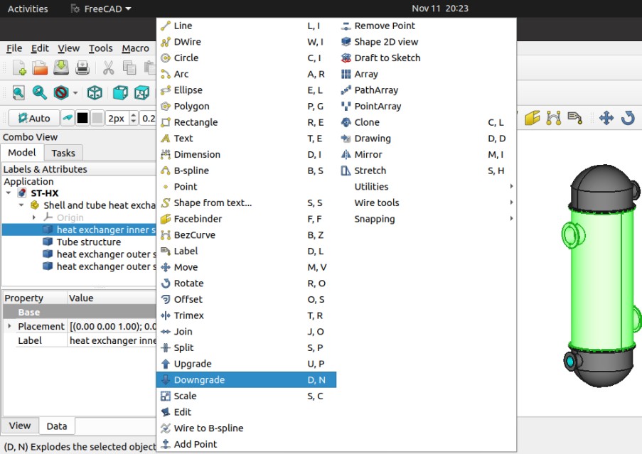
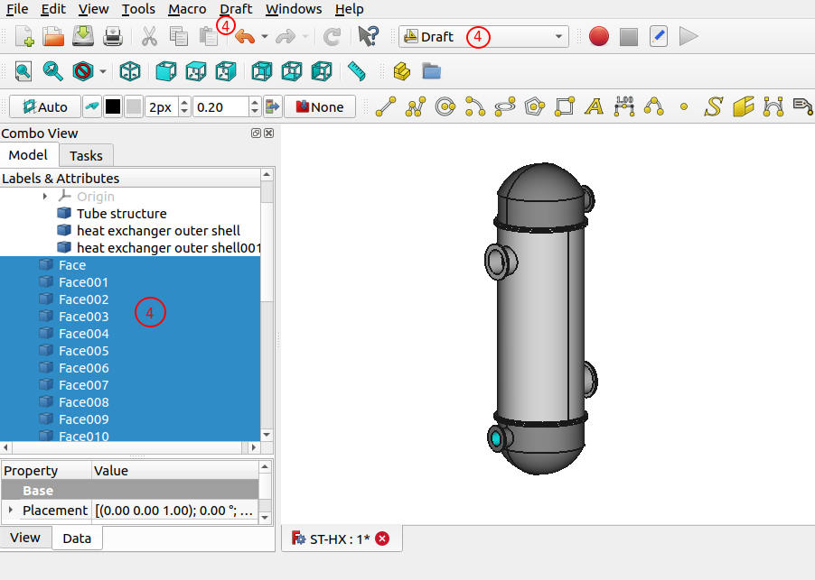
Python code to create a Heat Sink in FreeCAD
import FreeCAD as App
import Part
doc = App.newDocument("Heat_Sink")

# User Inputs: all length dimensions are in (mm)
fin_offset     = 2.5
fin_height     = 25
fin_thickness  = 3.0
fin_spacing    = 6.0
fin_num        = 10
base_width     = 80.0  # Y-direction, Length: X-direction, Height: Z-direction
base_thickness = 5.0

base_length    = (fin_num - 1) * (fin_thickness + fin_spacing)
base_length    = base_length + 2 * fin_offset + fin_thickness

# Create Base Plate and Fins
fin_base = Part.makeBox(base_length, base_width, base_thickness)
fins = []

for i in range(fin_num):
  x = fin_offset + i * (fin_thickness + fin_spacing)
  fin = Part.makeBox(fin_thickness, base_width, fin_height)

  fin.translate(App.Vector(x, 0, base_thickness))
  fins.append(fin)

# Combine All Solids and Display the Body
heat_sink = fin_base
for fin in fins:
  heat_sink = heat_sink.fuse(fin)

# heat_sink = heat_sink.makeFillet(1.0, heat_sink.Edges)

Part.show(heat_sink)
doc.recompute()
# Part.export([Part.show(heat_sink)], "Heat_Sink.step")
The content on CFDyna.com is being constantly refined and improvised with on-the-job experience, testing, and training. Examples might be simplified to improve insight into the physics and basic understanding. Linked pages, articles, references, and examples are constantly reviewed to reduce errors, but we cannot warrant full correctness of all content.
Template by OS Templates