CFD and Open-source!
OpenFOAM is free both for personal and commercial use […]

CFD stands for Computational Fluid Dynamics - the branch of mechanical engineering dealing with Fluid Flow and Heat Transfer. Whether you are a fresh graduate with engineering degree or a seasoned professional with industry and design background, you will find plenty of technical stuffs on CFD analyses and CFD software (both commercial such as FLUENT, CFX, STAR-CCM+ and COMSOL as well as open-source Gmsh, OpenFOAM, Salome and ParaView) online. This page is an attempt to provide all relevant information in one place and organized into logical steps. ::: Go to Table of Contents
How many of these names have you heard of? Click on the names to know more about them!

For flow and thermal simulation jobs, consultancy, training, automation and longer duration projects, reach me at  . Our bill rate is INR 1,200/hour (INR 9,600/day) with minimum billing of 1 day. All simulations shall be carried out using Open-source Tools including documentations.
Step-by-step guide to CFD, Mesh Generation and OpenFOAM!
CFD simulations methods are explained with features of OpenFOAM and ANSYS CFX / FLUENT, STAR-CCM+ and COMSOL. Applications related to turbo-machines, multi-phase flows, aero-acoustics ... have been described along with turbulence modeling and verification of results.
Werner Heisenberg: When I meet God, I am going to ask him two questions: why relativity? And why turbulence? I really believe he will have answer for the first! […]
OpenFOAM is free both for personal and commercial use […]
Modeling of the eddies where kinetic energy is lost through viscous dissipation […]
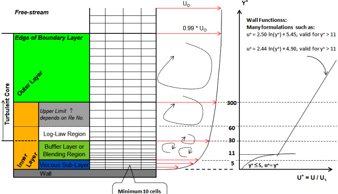
Boundary layers govern CFD simulation results. Know more about y+[…]
Logistic Regression, Decision Tree, SVM, Naive Bayes, KNN, Python, scikit-learn […]
Thermal simulations of electronic parts […]
Meshing is 50% capability, 50% art! […]
Flow in turbomachines: MRF, SMM, DMM […]
JS, PHP, MySQL […]
Some facts and sarcasms on corporate life […]
Theory and options in FLUENT / OpenFOAM […]
Tips and Tricks! […]
Guidelines on checking correctness of result! […]
Basic settings in FLUENT and OpenFOAM […]
AI in CFD: NVIDIA PhysicsNeMo (is an actively maintained) open-source deep-learning framework for building, training, and fine-tuning deep learning models using state-of-the-art Physics-ML methods. Refer link: github.com/NVIDIA/physicsnemo. A particular example on datacenter can be found in folder github.com/NVIDIA/physicsnemo/ tree/ main/ examples/ cfd/ datacenter. As per readme: "Thermal and airflow surrogate model for Datacenter design --- This example demonstrates the use of a Deep Learning model (3D UNet) for training a surrogate model for datacenter airflow to enable real-time datacenter design. The aim of this workflow is to train a Deep Learning model that can predict the temperature and airflow distribution within a hot aisle of a typical datacenter. For any given geometry of the hot aisle (height, width, and length) and the number of IT racks inside it, the trained model can predict the temperature, velocity, and pressure distribution inside the hot aisle instantaneously. Such an approach can be very useful from a datacenter design perspective where iterating through various design combinations is crucial to obtain optimal cooling and minimize hotspots."
It further explains: "Dataset - The model is trained on OpenFOAM simulation data. Based on the variables, i.e. Length, Height, Width, and Number of Racks, several hot aisle configurations are generated. These configurations are solved with OpenFOAM assuming maximum flow rate and rack exit temperature (max load condition). Steady state simulations are used and the resulting OpenFOAM data is exported in VTK format for training of the AI surrogate. The dataset is then normalized using the mean and standard deviation statistics of the dataset."How do we approach flow and thermal simulations? What steps one need to follow to make first time right (FTR) solution? These are some of the questions which have been answered in following sections with references to multiple pages covering each topic such as Mesh Generation, Boundary Conditions and Turbulence Modeling. For beginners to experienced users, the checklists are needed to ensure correct results and few sample checklists have been created.
It is imperative to have good understanding of mathematical methods adopted to solve linear system of equations, role of relaxation factors in iterative methods and rate of convergence. This has been explained clearly for a simple equation which is valid for any complex set of equations.
The table below summarizes few key pointers to define sound and quantifiable scope of CFD simulations. These are some of the topics which will lead the concerned stakeholders towards a well-thought scope. However, it may look a bit intimidating and intent is not to insist on all the information right at the beginning of the simulations. One key probing question to get insight into probable scope is to ask question: "At what stage the project is?" Budget planning, concept design, detailed design, prototype development?
| Topic | Description of requirement | Examples | Response |
| Objective | What is the primary aim? | Performance evaluation, Capacity upgrade, Design validation, Field failure, Safety, Emission | ? |
| Problem statement | What is expected output from CFD simulation? | Δp, Temperature, Flow uniformity, Heat flux, Volume fraction, Air-borne noise, Stagnant zone | ? |
| Prior investigation | What information is available from past or ongoing study? | Test report, Performance values, Field data, Hand calculations | ? |
| Geometrical details | What geometrical data is available for area of interest? | 2D drawing, 3D CAD data, Site images, Concept sketches | ? |
| Working fluid | Water, Air, Non-Newtonian, Mixture (Liquid-Solid, Liquid-Gas, Gas-Gas) | Homogeneous mixture, Two-phase flow, Emulsification, Stirred tank | ? |
| Time Domain | Steady (not dependent on time) or Transient (p, v, T vary with time) | Warm-up, cool-down, moving walls, varying flow rate | ? |
| System or Component | Is this a component level or system level simulation? | [Comp. level]: pump, fan in ducts, PCB [Sys. level]: Engine cooling system, Data centre | ? |
As mentioned earlier, it may look like a daunting task for a person not familiar with finer details of numerical simulations. Hence, a generic list of ingredients needed for CFD simulations can be used to start the discussion. This is summarized below.

A typical division of a CFD simulation or as a matter of fact any numerical simulation is in 3 categories namely Pre-Processing, Solution and Post-Processing. However, for beginners into this field, it does not convey much insight. The complete simulation process is explained here in a step-by-step sequence to make it easy to understand.


All these steps have been explained through an example simulation for "Flow Over a Back-Step" and can be found here! If you have access to ANSYS FLUENT, a step-by-step guide with GUI screenshots can be found in this PDF file. Similarly, if you have experience in using any commercial tool say CFX and want to try open-source product such as OpenFOAM, a comparison of methods is summarized in this page.
In addition to the steps, as a thermal and fluid flow analyst, you may need to make many other considerations as summarized below.
This is one of the most talked about (and sometimes dreaded) term used in numerical simulation field. The term 'convergence' refers to the process where the iterative method moves towards "expected final result". It is best explained using a problem from algebra where we need find out value of x in equation y = 5x2 + 25 when y = 1000. We all know a direct method:
x = [(y - 25)/5]0.5
Let's try an iterative method using algorithm xi+1 = xi × (1 - Δyi). Here, i refers to the iteration number and Δy refers to deviation of the calculated value of y from desired value of y = 1000, Res-Norm-1 refers to the absolute value where the residual % is normalized (divided) by the residual % obtained in 0th iteration based on guess value, Res-Norm-3 refers to the absolute value when the residual % is normalized (divided) by the residual % obtained in 0th ~ 2nd iterations.
| Iteration, i | xi | yi | Δyi | Res-Norm-1 | Res-Norm-3 | |
| Initial Guess | 10.00 | 525.0 | +475.0 | +47.5% | - | - |
| 1 | 14.75 | 1112.8 | -112.8 | -11.3% | 0.2375 | - |
| 2 | 13.09 | 881.2 | +118.8 | +11.9% | 0.2501 | - |
| 3 | 14.64 | 1096.7 | -96.70 | -9.67% | 0.2036 | 0.6032 |
| 4 | 13.22 | 899.45 | +100.6 | +10.1% | 0.2117 | 0.6272 |
| 5 | 14.55 | 1084.1 | -84.14 | -8.41% | 0.1771 | 0.5248 |
| 6 | 13.33 | 913.40 | +86.60 | +8.66% | 0.1823 | 0.5401 |
| 7 | 14.48 | 1073.9 | -73.93 | -7.39% | 0.1556 | 0.4611 |
| 8 | 13.41 | 924.57 | +75.43 | +7.54% | 0.1588 | 0.4705 |
| 9 | 14.42 | 1065.4 | -65.40 | -6.54% | 0.1377 | 0.4079 |
| 10 | 13.48 | 933.77 | +66.23 | +6.62% | 0.1394 | 0.4131 |
| 11 | 14.37 | 1058.1 | -58.14 | -5.81% | 0.1224 | 0.3626 |
| 12 | 13.54 | 941.50 | +58.50 | +5.85% | 0.1232 | 0.3649 |
| 13 | 14.33 | 1051.9 | -51.86 | -5.19% | 0.1092 | 0.3235 |
| 14 | 13.59 | 948.11 | +51.89 | +5.19% | 0.1092 | 0.3236 |
| 15 | 14.29 | 1046.4 | -46.39 | -4.64% | 0.0977 | 0.2894 |
| 16 | 13.63 | 953.82 | +46.18 | +4.62% | 0.0972 | 0.2881 |
| 17 | 14.26 | 1041.6 | -41.59 | -4.16% | 0.0876 | 0.2594 |
| 18 | 13.67 | 958.79 | +41.21 | +4.12% | 0.0868 | 0.2570 |
| 19 | 14.23 | 1037.3 | -37.34 | -3.73% | 0.0786 | 0.2329 |
| 20 | 13.70 | 963.15 | +36.85 | +3.68% | 0.0776 | 0.2298 |
| 21 | 14.20 | 1033.6 | -33.56 | -3.36% | 0.0707 | 0.2094 |
| 22 | 13.73 | 967.00 | +33.00 | +3.30% | 0.0695 | 0.2059 |
| 23 | 14.18 | 1030.2 | -30.20 | -3.02% | 0.0636 | 0.1884 |
| 24 | 13.75 | 970.40 | +29.60 | +2.96% | 0.0623 | 0.1846 |
| 25 | 14.16 | 1027.2 | -27.19 | -2.72% | 0.0572 | 0.1696 |
Look how the calculated value of x still makes y off the final value by 2.72% even after 25 iterations. What are the ways to speed-up this process - that is how can we reach to the correct value with lesser number of iterations? One option is to change the way the value of xi+1 is calculated from xi. This method is known as use of "Relaxation Factors" in numerical simulation technology. Let's try the approach: 0.8 in the following equation is the relaxation factor (also called under-relaxation factor as the value is < 1.0).
xi+1 = [xi × (1 - Δyi)] * 0.8 + xi * 0.2
| Iteration, i | xi | yi | Δyi | Res-Norm-1 | Res-Norm-3 | |
| Initial Guess | 10.00 | 525.0 | 475.0 | 47.5% | - | - |
| 1 | 14.75 | 1112.8 | -112.8 | -11.3% | 0.2375 | - |
| 2 | 13.42 | 925.30 | +74.70 | +7.50% | 0.1572 | - |
| 3 | 14.22 | 1036.1 | -36.11 | -3.61% | 0.0760 | 0.2480 |
| 4 | 13.81 | 978.54 | +21.50 | +2.10% | 0.0452 | 0.1474 |
| 5 | 14.05 | 1011.6 | -11.56 | -1.16% | 0.0243 | 0.0794 |
| 6 | 13.92 | 993.39 | +6.61 | +0.66% | 0.0139 | 0.0454 |
| 7 | 13.99 | 1003.7 | -3.66 | -0.37% | 0.0077 | 0.0251 |
| 8 | 13.95 | 997.94 | +2.06 | +0.21% | 0.0043 | 0.0141 |
| 9 | 13.97 | 1001.1 | -1.15 | -0.11% | 0.0024 | 0.0079 |
| 10 | 13.96 | 999.35 | +0.65 | +0.06% | 0.0014 | 0.0044 |
| 11 | 13.97 | 1000.4 | -0.36 | -0.04% | 0.0008 | 0.0025 |
| 12 | 13.96 | 999.80 | +0.20 | +0.02% | 0.0004 | 0.0014 |
| 13 | 13.97 | 1000.1 | -0.11 | -0.01% | 0.0002 | 0.0008 |
| 14 | 13.96 | 999.94 | +0.06 | +0.01% | 0.0001 | 0.0004 |
| 15 | 13.96 | 1000.0 | -0.04 | +0.00% | 0.0001 | 0.0002 |
| 16 | 13.96 | 999.98 | +0.02 | +0.00% | 0.0000 | 0.0001 |
| 17 | 13.96 | 1000.0 | -0.01 | +0.00% | 0.0000 | 0.0001 |
This is an excellent example of relaxation factor improving the speed of convergence. Readers are advised to try out the calculation with different values of initial guess (say 12, 15 instead of 10) and relaxation factor (say 0.2, 0.5 instead of 0.8) to see the effect on rate of convergence (number of iterations required to find result x = 13.96).
A*xP + B*xN + C*xS + D*xE + E*xW = FP where P denotes the calculation node and N, S, E, W denotes the north, south, east and west nodes respectively. Here, absolute residual is
εn = [A*xPn + B*xNn + C*xSn + D*xEn + E*xWn - FPn] where n is the iteration number.
A checklist and comparison sheet should be used when a new design is worked out or major upgrades in designs are under considerations.
| S. No. | Performance Indicator | Baseline | Upgrade |
| 1 | Pressure drop | ≤ 2.0 [kPa] | ≤ 1.5 [kPa] |
| 2 | Temperature rise | ≤ 15 [K] | ≤ 12 [K] |
| 3 | Wetted surface area | ≥ 1.0 [m2] | ≥ 1.5 [m2] |
| 4 | Capacity or volumetric size | ≤ 5.0 [cm3] | ≥ 7.5 [cm3] |
| 5 | Power consumption | ≤ 50 [W] | ≤ 40 [W] |
Application of CFD in terms of physics, application and industry: sophisticated computer-based analysis technique to evaluate various design alternatives, identify flow and temperature problems, develop solutions and formulate physical validation strategies. Troubleshoot existing design, generate smarter solutions and more optimized design with shorter development cycle to meet ever-increasing demands of working performance and environmental concerns.
| S. No. | Simulation Category | Physics | Application | Industry |
| 01 | Basic |
|
| Automotive, FMCG, Aerospace, Recreational Vehicles, Data Centres, Valves |
| 02 | Rotating Devices |
|
| Automotive, Home Appliances, Whitegoods, Pharmaceuticals, FMCG, Dairy Industry |
| 03 | Multi-phase Flows |
|
| FMCG, Buildings and Real-Estate, Oil and Gas Industry, Medical Devices, Pharmaceuticals |
| 04 | Advanced Methods |
|
| Aerospace, Combustion Engines, Turbines, Automotive, Off-Highway Vehicles, Recreational Vehicles, Heat Recovery Devices, Car Parking, Road Tunnels |
| 05 | Multiphysics |
|
| Medical Devices, Elevators, Aerospace, Automotive, Burners / Combustors |
| 06 | Electronic Cooling |
|
| Home Appliances, Whitegoods, ICEPAK, FloTHERM, Sigma Technologies |
This list is no way unique and can be arranged in too many ways to suit specific purpose. The attempt is to cover entire gamut of application in a short yet detailed manner.
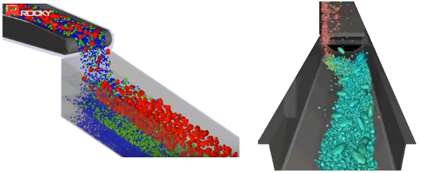
Discrete Element Method: The well-known FEM and FVM method are continuum-based calculation techniques where the medium is assumed to conform to continuum hypothesis (the properties of the matter are considered as continuous functions of space variables x, y an z). Though all matters are composed of atoms and molecules, the concept of continuum assumes a continuous distribution of mass within the matter with no void or empty space.
ROM stands for Reduced Ordered Modeling which is an attempt to expedite the simulation speed with some compromise in accuracy. This is also known as MOR (Model Order Reduction). At the very basic level, ROMs can be the simplification of full 3D simulations to smaller equivalent domains such as 2D section, symmetric and periodic domains. One of the high fidelity ROM is simulation of flow through pipe as a rectangular plane than can be rotated about one of its longer sides to create the full cylinder. Though not all industrial applications can be simplified to this extent!
Reduced order modeling is a fairly generic term and the semantics changes from field to field (e.g. computer science, mechanical engineering, testing...) and includes all methodologies and algorithms that aim to reduce the complexity of a problem.
Excerpt from web.stanford.edu/group/frg/active_research_themes/reducedmodel.html: "Reduced-order models (ROMs) are usually thought of as computationally inexpensive mathematical representations that offer the potential for near real-time analysis. While most ROMs can operate in near real-time, their construction can however be computationally expensive as it requires accumulating a large number of system responses to input excitations."
As per mathworks.com/discovery/reduced-order-modeling.htm: Many techniques such as singular value decomposition (SVD), eigenvalue decomposition (EVD), principal component analysis (PCA), lookup tables, interpolation and curve fitting are also useful as part of model order reduction. As per in.mathworks.com/discovery/reduced-order-modeling.html - "Reduced order modeling (ROM) and model order reduction (MOR) are techniques for reducing the computational complexity or storage requirement of a computer model, while preserving the expected fidelity within a controlled error. Working with surrogate models can simplify analysis and control design. Scientists and engineers use ROM techniques to create system-level simulations, design control systems, optimize product designs, and build digital twin applications."
Excerpts from "An Overview of Reduced Order Modeling Techniques for Safety Applications" by D. Mandelli et. al. The safety modeling of a nuclear system is not only a thermal-hydraulic problem but several other models are required: neutron transport, thermo-mechanics, chemistry, fracture propagation... Note how the overall problem is not only multi-physics but also multi-scale both in the spatial scale but also in the temporal scale. The concept of Reduced Order Modeling can be categorised into three main categories:
Machine Learning (ML) in Numerical Simulations: It is proven that Monte Carlo method can be used to solve Conduction Equation without mesh generation and matrix inversion. However, same does not apply to FEA or CFD. Any ML and/or ANN (Artificial Neural Network) does not solve the underlying physics - they act as what is called "surrogate models" to work on the data generated by FEA or CFD or any numerical simulations, play the role of a decision maker. In case of Fluid Dynamics, ANN cannot be even a surrogate model to turbulence modeling (please note the word 'modeling' after turbulence) because if turbulence can be predicted, numerically computed or interpolated, the methods of CFD simulations would not remain worthy of a ML or NN.
Fluid-Structure Interaction - this is a multi-physics application of CFD methods where the effect of fluid forces cause deflection of the structure large enough to affect the flow field. Thus, it is a two-way coupling where CFD and FEM method need to share the information to define time-dependent displacement of walls and fluid velocity/pressure fields. As evident, this is necessarily an unsteady (transient) phenomena and selection of time step is crucial and most of the times not known a-priori. Application includes dynamic response of reed valves in a hermetically sealed reciprocating compressor, motion of swing check valve in water pipelines, equilibrium position of check valves...
Excerpts from Fluid-Structure Interaction (FSI) case study of a cantilever using OpenFOAM and DEAL.II with application to VIV, Johan Lorentzon, June 17, 2009: The Fluid-Structure Interaction (FSI) appears as a physical phenomenon in engineering such as static load, drag, and Flow-Induced Vibrations (FIV) or Flow-Induced Pulsations (FIP). FIV is further classified into flutter, galloping and vortex-induced vibrations (VIV). The static load on the structure originates mainly from the total pressure difference between front and wake side of the structure. The dynamic pressure can, due to instability in the structure where the damping is less than the energy transferred by the vortex-induced wake, create a resonance with the structure with a negative damping known as flutter. Typical examples of applications in which flutter is considered are aircraft wings, tall buildings, rotating blades and long-span bridges. The VIV concerns bridges, chimneys, heat exchanger tubes, power lines and undersea constructions such as sea cables/risers or biomechanical applications as blood vessels.
Reference: Flow Induced Pulsations Caused By Split Flow In A T-Branch Connection by Stefan P.C. Belfroid et al. ASME 93884 - "By using a vortex blob method it has been demonstrated that cross flows even up to 25% of the main flow lead to significant FIP source strength. With increasing cross flow merging from the side branch into the main flow, the maximum source strength shifts to slightly lower Strouhal number due to the increased convective velocity of the vortex structures. The source strength decreases rapidly for increasing cross flow. As a rule of thumb, the source strength becomes negligible for cross flows larger than 25% of the total flow."
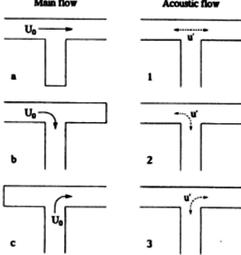
When the mean flow is diverted completely into the side branch (case 'b') no pulsating flow is encountered. However, for cases 'a' and 'c', strong pulsations have been measured. For calculating acoustic resonances of a piping system, one dimensional simulation tools are quick and reasonable accurate. A full acoustic solution including travelling and standing waves can be carried out in the flow system.
Computational Aero-Acoustics - this is another multi-physics application of CFD methods to predict the noise sources and solve noise propagation using other solvers such as ACTRAN. In CFD simulation environment, acoustics is just a post-processing activity where the fluctuating component of pressure is converted into noise using density-based analogies like (Lighthill’s analogy, Powell’s analogy, the Ffowcs Williams–Hawkings [FWH] analogy and Curle’s analogy) or few other analogies like Phillips’ analogy and Lilley’s analogy, Howe’s analogy and Doak’s analogy. The noise source can be calculated both for steady and transient turbulent flows, however the option available will vary for steady state and transient cases.
Boundary Element Method - also known as the "boundary integral equation method" or "boundary integral method": As the name suggest, this method discretizes only the boundaries of the computational domain. Widely used in field problems with unbounded exterior domain but bounded boundaries such as magnetic field calculation and acoustics - this method does not need to model the entire domain required in FEM/CFD.
Magneto-Hydro-Dynamics (MHD) or Hydro-Magnetics is the physical-mathematical macroscopic theory that deals with dynamics of magnetic fields in electrically conducting fluids [plasma, liquid metals, salt water and electrolytes]. It does not apply to effect of magnetic field on fluids containing magnetic particles. The presence of magnetic fields leads to forces that in turn act on the fluid thereby potentially altering the topology and strength of the magnetic fields themselves.
The set of equations that describe MHD are a combination of the Navier–Stokes equations of fluid dynamics and Maxwell’s equations of electromagnetism. These differential equations have to be solved simultaneously, either analytically or numerically.
The study of ferromagnetic particle suspensions is relevant for better understanding of wet-state separation processes in mineral processing and recycling. Stokesian dynamics is a particle-based, mesh-free method developed for nm to mm size particles in static or flowing liquid suspensions. LB-LES-DEM approach (Lattice-BoltzmannLarge Eddy Simulation-Discrete Element Method) has been investigated to evaluate the combined effect of liquid phase flow and magnetic effects though limited number of particles can be used due to the high computational cost.
Lattice Boltzmann Method - a discrete computational method based on Boltzmann's equation. This is an alternate method to make fluid dynamics simulations based on lattice gas methods. The method allows particles to move on a discrete lattice (analogous to mesh) and collide such that local collisions conserve mass (continuity) and momentum (Navier-Stokes equation).
Excerpts: "High fidelity transient Lattice Boltzmann based solution, accurate across most flow regimes (laminar to transonic) to solve the most complex CFD design problems in Transportation & Mobility and Aerospace & Defence."
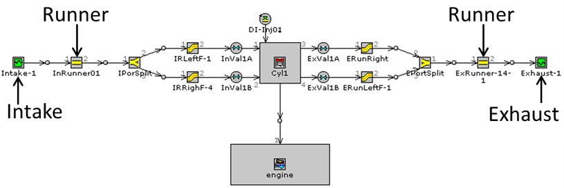
Fluid Network Method - a flow and pressure drop calculation approach based on analogy with electric resistances and circuits. 3D flow paths are condensed into equivalent flow resistance 'R' defined as Δp = ρ × R × Q2 where Q is flow rate. A network is created with nodes and branches where nodes represent the connection of two or more branches (the flow resistances). Similar to Kirchhoff's law for electrical networks, the flow and pressure drop across each hydraulic resistance can be calculated using mass balance at each node and zero pressure drops across all the flow loops. Hardy-Cross method is one of the widely used method to solve flow network models. 1D model for a single cylinder engine in GT-Power described below is an example of FNM.

Excerpts - "The Modelica Language is a non-proprietary, object-oriented, equation based language to conveniently model complex physical systems containing, e.g. mechanical, electrical, electronic, hydraulic, thermal, control, electric power or process-oriented subcomponents."
DYMOLA (DYnamic MOdelling LAboratory) is a user interface and Modelica language compiler owned and developed solely by Dassault Systems. DYMOLA enables the user to write, compile and simulate Modelica based models. There are other Commercial Modelica Simulation Environments such as ANSYS Simplorer, SimulationX from ESI ITI GmbH and Simcenter Amesim from Siemens. There is an open-source and free simulation environment tool for Modelica named OpenModelica.
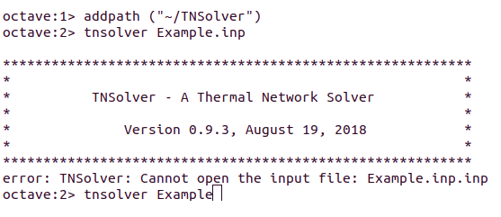
RELAP5: Reactor Excursion and Leak Analysis Program, developed at Idaho National Laboratory for the U.S Nuclear Regulatory Commission, is widely used 1D codes in the nuclear industry.TNSolver: The Open Source Thermal Network solver written in GNU Octave can be found at heattransfer.org/TNSolver. To run it, follow the commands shown below. Note that you do not need to specify the input file with extension .inp. The path to TNsolver folder needs to be added to every GNU Octave session.
The paper "Steady Flow Analysis of Pipe Networks: An Instructional Manual" by Roland W. Jeppson describes the Python code to solver fluid networks. Python Library for Fluid Mechanics is available at github.com/CalebBell/fluids. The repository contains Python codes to calculate friction factors, loss coefficients in fittings and valves, drag coefficients for bluff bodies, pressure drop across packed beds, mixing of fluids...
SU2 stands for Stanford University Unstructured. This is an open-source solver having its own mesh format. The other way to interact with SU2 is to use of CGNS for mesh and ParaView / Tecplot for post-processing. The work-flow of SU2 is as follows. It is a text-based solver similar to OpenFOAM where a single configuration file is equivalent to the 0, controlDict, transportProperties and fvSolution dictionaries. A converter from CGNS to the SU2 format has been built into SU2 and hence the mesh does not need to be explicitly converted into SU2 format.
| Simulation Activity | Method |
| Mesh Generation | SU2 can be used to generate for simple shapes. For most practical operations,mesh has to be generated in other pre-processors such as OpenFOAM, GMSH, Pointwise, ICEM CFD... |
| Convert mesh into SU2 format | GMSH and CENTAUR can save the mesh directly in SU2 format. The Python script written by Laurent Berdoulat can be found here to convert OpenFOAM mesh into SU2 format. The input file template for 2D meshes is here and the input file template for 3D meshes is here. |
| Convert mesh into SU2 format | For commercial programs, name boundaries (used as marker tags in SU2) appropriately before exporting the mesh into CGNS format. Use MESH_FORMAT= CGNS* in configuration file. |
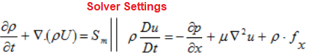
| Solver Setting | Define material, apply boundary conditions, select solver type, set iteration controls and relaxation factors... as per pre-defined format in a configuration file. |
| Post-processing settings | Set the output format for results: OUTPUT_FORMAT= TECPLOT or OUTPUT_FORMAT= PARAVIEW, OUTPUT_FILES = PARAVIEW_ASCII |
| Make the simulation run | F:\SU2\SU2_CFD.exe wedgeShock.cfg, for parallel computing: mpirun -n 8 SU2_CFD.exe wedgeShock.cfg or use Parallel Computation Script - parallel_computation.py |
| Result Files | flow.dat or flow.vtk - full volume flow solution |
| surface_flow.dat or surface_flow.vtk - flow solution along the wall surfaces | |
| surface_flow.csv - file containing values along the wall surfaces | |
| restart_flow.dat - restart** file in an internal format for restarting this simulation in SU2 | |
| history.dat or history.csv - file containing the convergence history information | |
| SU2_CFD (Computational Fluid Dynamics Code): Solves direct, adjoint and linearized problems for the Euler, Navier-Stokes, and Reynolds-Averaged Navier-Stokes (RANS) equation sets, among many others. | |
| SU2_DOT (Gradient Projection Code): Uses the surface sensitivity, the flow solution and the definition of the geometrical variable to evaluate the derivative of a particular functional (e.g. drag, lift...). | |
| SU2_DEF (Mesh Deformation Code): Computes the geometrical deformation of an aerodynamic surface and the surrounding volumetric grid. Once the type of deformation is defined, SU2_DEF performs the grid deformation by solving the linear elasticity equations on the volume grid. | |
| SU2_MSH (Mesh Adaptation Code): Performs grid adaptation using various techniques based on an analysis of a converged flow solution, adjoint solution and linearized problem to strategically refine the mesh about key flow features. | |
| SU2_SOL (Solution Export Code): Generates the volumetric and surface solution files from SU2 restart files. | |
| SU2_GEO (Geometry Definition Code): Geometry preprocessing and definition code. In particular, this module performs the calculation of geometric constraints for shape optimization. | |
*SU2 will not use any specific boundary conditions that are embedded within the CGNS mesh. However, it will use the names given to each boundary as the marker tags.
**The restart files can be used as input to generate the visualization files using SU2_SOL module. This will be done automatically if the parallel_computation.py script is used, but it can also be done manually at any time by calling SU2_SOL.
This is a special type of transient phenomena which calculates pressure generated due to sudden change in flow velocity and subsequent calculation of pressure wave propagation. Pressure waves can be caused by e.g. valve operations, pump trips, pipe break and loss of liquid. Hence, computations related to water hammer involves both CFD and wave speed calculation techniques. Suppose water is flowing into a straight long pipe at constant flow rate and suddenly a control valve is use to reduce the flow rate by 50% or even stopped the flow completely, a pressure wave will get generated which will travel upstream at a speed closer to speed to sound in water. This phenomena is governed by Joukowsky equation: Δp = [± ρ c Δv] where ρ is the density of fluid, c is (water-hammer) wave speed and δv is change in velocity. Similarly, a pump tripping or shut-down is equivalent to valve closure which also causes water hammer - which is equivalent to opening of a control valve to increase the flow rate in the pipe. Note:
This is known as fundamental equation of water hammer. Thus, head developed due to water hammer, Δh = [c Δv / g] where g is acceleration due to gravity. This is inherently a transient phenomena and CFD methods require simulation for steady state condition and then implementation of a transient phenomena over a converged steady state flow field. In industry, there are many 1D tools which are based on Methods of Characteristics (MOC) to solve water hammer phenomena. Some of the tools are WANDA, HAMMER, AFT Impulse... In CFD simulations, valve closure can be modeled either by changing geometry or by decreasing the mass outflow of the pump or piping system.
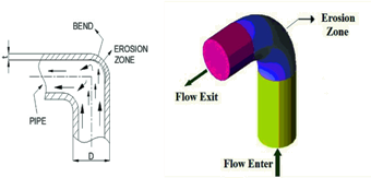
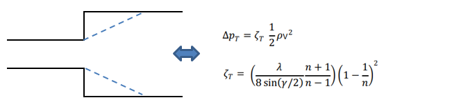
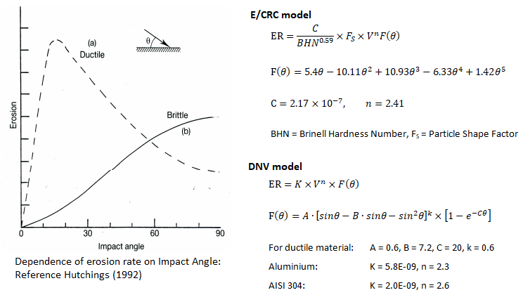
[Image Reference: Springer] Loss of material due to impact of solid particles. For example, sand particles hitting at high velocity of a solid wall causing loss of material by "cutting or chipping mechanism" and/or by "deformation mechanism". Erosion may also occur by abrasive process where particle slip along the wall causing rubbing action between particles and the wall. Erosion can also occur due to cavitation and liquid particle drop falling over a wall. The erosion rate is function of impact velocity, impact angle, particle properties (sharpness ratio), hardness of the wall and hardness of the solid particle. Experiments have shown that there is exponential correlation between particle impact velocity and rate of erosion.
The erosion process is not a mathematically well-defined problem and the estimation of erosion location as well as erosion rate relies heavily on empirical correlations such as erosion rate E = C × FS × Vn × F(θ) where C and n are constants, FS is a particle shape factor (~1.0 for particles with sharp corners say diamond, cone and square shapes, ~0.5 for semi rounded shapes such as cylinders, disks and ellipsoids and ~0.2 for fully rounded shapes such as spheres). V is impact velocity and F(θ) is impact angle function. The "paint erosion test" is a quick and reliable approach to find "erosion pattern". It is analogous to measurement of contact area for bolted joints.
Erosion modeling using CFD: This is a 3-step process described below.
CFD for Pneumatic Conveying Process: The viscous and pressure forces cause the particles to move against friction and gravity. The minimum velocity required to make the particles move is called "particle pick-up velocity". Saltation velocity is the value at which majority of the solids become entrained in the airstream. Air volume flow rate optimization is the critical process to achieve smooth conveying without slugging and plugging of the conduits. The conveying process also has to deal with "dilute phase" (air velocity > saltation velocity, suspension flows) and "dense phase" (air velocity < saltation velocity) conveying. The dilute and dense phases are also distinguished by solid loading (volume or mass fraction of the solids). The assessment of conveying capacity is similar to multiphase flow simulation where the solid phase is treated as continuum. Applications includes conveying of coffee beans, grains, granular sugar, cement powder, lime, spices...
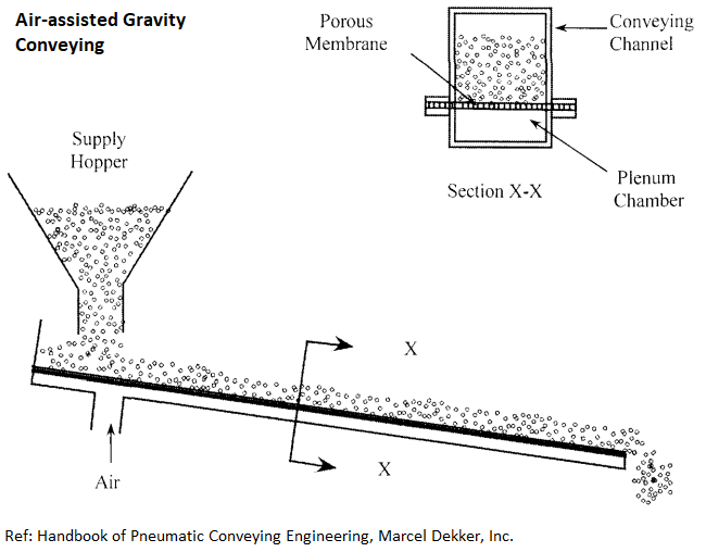
Choking Velocity - This equals the actual gas velocity in a vertical pipeline at which particles in a homogeneous mixture with the conveying gas settles out of the gas stream. Bulk Density (Fluidized) - it is the apparent (equivalent) density of a material in its fluidized or suspension state. It is generally lower than either the packed or loose bulk density due to the air absorbed into the voids. Angle of Repose - The angle of repose of a material is the angle formed between the horizontal and sloping surface of a piled material, which has been allowed to form naturally without any conditioning. This helps estimate the slope of the channel for gravity assisted conveying. Terminal Gas Velocity - The terminal gas velocity in a pneumatic conveying system is the velocity of the gas as it exits the system. It is also known as the ending gas velocity and conveying line exit velocity. Floodability - describs the tendency of a material to aerate and act as a fluid, squeeze material quickly in your fist - if it squirts through fingers, then it is floodable. Floodable materials are difficult to restrain in controlled feeding applications. Pneumatic Conveying Design Guide by David Mills is another good reference to start with.
The near- and far-field break-up and atomization of a liquid jet (aerodynamic break-up of liquids) in multi-phase fluid systems fits in the broader category of multi-phase fluid flow. Jet and spray formation has many applications such as inhalers in medical applications, fire-extinguishers, Diesel engines, water chillers... Primary atomization of the liquid jet occurs near the outlet of the nozzle. Turbulent fluctuations of the liquid jet induce perturbations on the jet surface, which grow and break the jet into droplets. The length scale of turbulence is the dominant length scale of atomization, which also determines the resulting droplet size (Chryssakis et al.)1.
2In the plain-orifice atomizer model, the operation mode of the nozzle is determined based on the Reynolds number, the cavitation number and the critical values for the inception of cavitation and flipping (ANSYS, 2016). The Reynolds number based on hydraulic head is defined as ReH = (D ρL / μ) [2(p1 − p2)/ρL]0.5 where D is the nozzle diameter, ρL is the liquid density and μ is the liquid viscosity. The upstream and downstream pressures are denoted by p1 and p2, respectively. The cavitation number is defined as K = (p1 − pv)/(p1 − pv) where pv is the vapour pressure of liquid at operating temperature. For short, sharp-edged nozzles, the inception of cavitation occurs approximately at cavitation number K ~ 1.9.1Chryssakis, C.A., Assanis, D.N. and Tanner, F.X., 2011. Atomization Models, in Handbook of Atomization and Sprays, Ed. N. Ashgriz, Springer, New York, USA.
2ANSYS Fluent Theory Guide, section Atomizer Model Theory
Additional information on Jet Break-up can be found here.
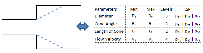
DOE in CFD Simulations: When CFD simulations are used to check impact of various parameters such as mesh size, turbulence model / wall function, inlet boundary condition, discretization scheme and P-V coupling, a Design-of-Experiments can be used to make the evaluation more scientific and robust. Here k = number of factors = 5. If each of these parameters considered are at two levels (two types or values), there are total 25 = 32 runs to be completed. It have been observed that the interactions involving > 3 factors are insignificant and a fractional factorial can be used. There is Python package PyDOE3 available to generate DOE tables, though a good understanding of DOE concepts are required to use it.
One of the key concept in both CFD and DOE is DOF (Degrees-of-freedom). In order to understand a classroom with capacity N. The first student has N choices to take a seat, the second student has N-1 options and so on. The last student will have no choice. Thus, in case of N dataset, the DOF is N-1.
A full quadratic model contains all main effects, all quadratic effects and all possible two-way interactions. For a set of k-factors, the number of terms in a full quadratic model is N = (k+1)(k+2)/2. Thus, for k = 4, N = 15 ad for k = 5, N = 21. Central Composite Design (CCD) and Box-Behnken Design (BBD) are used to reduce the number of terms. This is part of the family known as Response Surface Model (RSM) which looks for quadratic and/or higher order trends as well as assumes that all variables are significant.
The interactions are designated as main effects, 2-way interactions, 3-way interactions and so on. The number of runs for main effect = kC1 = k, number of runs for 2-way interactions = kC2 = k/2 × (k-1), number of runs for 3-way interactions = kC3 = k/6 × (k-1) × (k-2) ... This is also known as degrees-of-freedom where each main effect will have two degrees of freedom when each factor has three levels. Each two-factor interaction has (3−1) × (3−1) = 4 degrees of freedom. The ABC interaction has (3−1) ×(3−1)×(3−1) = 8 degrees of freedom.
When there is a curvilinear (non-linear) relation between the response and a quantitative factor, it is not possible to detect such a curvature effect with two levels. A mix-level design refers to experiments where factors have unequal levels. For example, factor A has two levels, factor B has 3 levels and factor C has 4 levels.
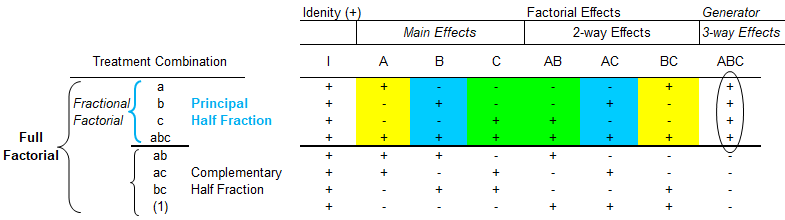
Two most important properties of any factorial designs are 'balance' and 'orthogonality'. Balance requires that each level of a factor is run the same number of times in an experiment. For example, a design with 4 factors, first with 2 levels, second with 3 levels, third with 4 levels and the last with 5 levels. To generate a balanced design, at least 60 runs are needed. Orthogonality refers to pairwise linearly independent columns, useful for assessing factor significance. In vector mechanics, two vectors are orthogonal if the dot product of the vector and hence the sum of the products of their corresponding elements is 0.
Let's consider an experiment that has 4 variables each at 3 levels. A full factorial experiment would require 34 = 81 experiments. A Taguchi experiment with a L9(34-2) orthogonal array will require only 9 runs. Thus, Taguchi's orthogonal arrays are highly fractional factorial designs. Here L9 means array requires 9 runs. All Taguchi's arrays are orthogonal but highly unbalanced.
| Run | Factor-A | Factor-B | Factor-C | Factor-D |
| 1 | 1 | 1 | 1 | 1 |
| 2 | 1 | 2 | 2 | 2 |
| 3 | 1 | 3 | 3 | 3 |
| 4 | 2 | 1 | 2 | 3 |
| 5 | 2 | 2 | 3 | 1 |
| 6 | 2 | 3 | 1 | 2 |
| 7 | 3 | 1 | 3 | 2 |
| 8 | 3 | 2 | 1 | 3 |
| 9 | 3 | 3 | 2 | 1 |
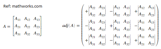
Adjoint: In linear algebra, Adjoint or Adjugate refers to conjugate transpose of a matrix. For a square matrix where inverse exists, AH ≡ adj[A] := Inverse[A] Det[A] An analogous concept applied to an operator instead of a matrix is also known as the Hermitian conjugate.The adjoint operator is widely used in both Sturm-Liouville theory and quantum mechanics.
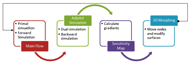
Optimization of shape and size in CFD simulations require incremental change in geometry and re-meshing. The CFD programs are now incorporating adjoint solvers which runs in addition to the fluid solver to find an optimum geometry to minimize (e.g. pressure drop) or maximize (e.g. flow uniformity) specified field variables. Both the Single Object Optimization (SOO) and Multiple Objectives Optimization (MOO) are possible.
Similar concepts Full Order Modeling (FOM) and Reduced Order Modeling (ROM) which are based on mathematical concepts such as MDO (Multidisciplinary Design Optimization), Higher Dimension Model (HDM), Proper Orthogonal Decomposition (POD) or Singular Value Decomposition (SVD).
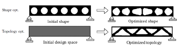
There are 4 types of optimization techniques:
| Optimization Method | Salient Features |
| 0D | Empirical |
|
| 1D | Parameter optimization |
|
| 2D | Surface or Shape Optimization |
|
| 3D | Topology optimization |
|
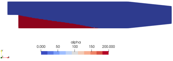
Excerpts from "Topology Optimisation of Fluids Through the Continuous Adjoint Approach in OpenFOAM" by Prof. Hakan Nilsson - "The Topology Optimization Method (TOM) consists in determine the material distribution in a design domain to maximize or minimize an objective function subject to certain constraints. To maximize/minimize the objective function at flow devices is done by adding the velocity field u multiplied by a scalar field α to the momentum equations, so regions with a high value of α determine a low permeability area (solid portion) and regions with a low value of α determine a high permeability area (fluid portion)." This paper AIAA-2007-3947 describes the implementation of topology optimization in OpenFOAM.
For incompressible steady state Navier-Stokes equations, the problem can be written as:minimize cost function J = J(U, p, α).
such that R ≡ (U . ∇)U + ∇p − ∇.[2μD(U)] + αU = 0, strain rate tensor D(ν) = ∇U + (∇U)T
∇.U = 0
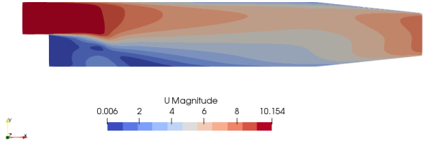
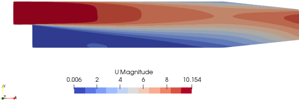
Note:Here, α is the porosity. In OpenFOAM, adjointShapeOptimizationFoam solves both the primal flow (U) and the adjoint flow (Ua) and at the same time optimizes the geometry for minimized cost function say pressure loss. The solver is built around a case of optimization of a duct shape by applying blockage in regions causing pressure loss which are estimated using the adjoint method. The solver is also programmed for shape optimization with respect to pressure loss. The redundant material is shown by high value of α (closer to alphaMax specified in transportProperties dictionary). A detailed description of adjointShapeOptimizationFoam solver can be found here. The pitzDaily case (flow over a back step with pinched outlet) gives following output:
Initial Velocity
Optimized Porosity
Optimized Velocity
 s
s
Excerpts from blogs.sw.siemens.com/simcenter/topology-optimization-cfd-creating-designs-like-nature:- The topology optimization method is based on a level set approach. Unlike the traditional porosity method this approach is not just blocking the flow from the cells with source terms. It is rather defining a moving interface around the predicted flow path. And, this has various advantages! Getting a cleaner interface between solid and fluid which results in designs with less kinks and folds. Eliminating the spare pockets of flow that the porosity method creates. This significantly reduces the clean-up and CAD reproduction time and ultimately reducing the cost of production.
Excerpts from NAFEMS paper "Adjoint-based Topology Optimization - Maximizing Heat Transfer of a Brake Cooling Duct" - Additive manufacturing has made it possible to push the limits of designs beyond the skills and imagination of traditional design engineers. Topology optimization closes the gap between the possibilities and the automation in obtaining those organic optimized shapes. A key class of engineering problems, fluid and thermal applications, are benefiting from the advances on those two design and manufacturing technologies.
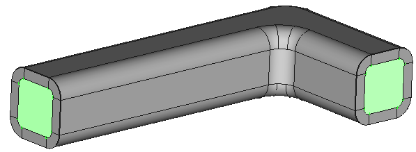
Shape Optimization using Mesh Deformation: The shape optimization process uses the morphing procedure to deform the geometry of interest. Specified control points are displaced by amounts calculated using mesh sensitivities that the adjoint solver provides. The displaced positions of the specified control points are set to maximize/minimize the cost function of interest. At each boundary of computational domain, the conditions of how should be morphed needs to be specified. E.g. the simulation of an airfoil within a wind tunnel, only the airfoil is subject to adjoint shape optimization with the vertices at the boundary being morphed. The surrounding wind tunnel boundaries remain fixed.
Advantage of Adjoint Methods
The adjoint method is an efficient means to predict the influence of many design parameters (inputs) on sensitivity of the objective (output). The advantages of the adjoint method are:SIMULIA Tosca Fluid: Shape Optimization for Fluid Flow
| Isight: Parametric Optimization | Tosca: Non-parametric Optimization |
| Size, shape and location of the cutout is known at the beginning and it is constrained by parameters | Size, shape and location of the cutout is unknown and thus is non-parametric optimization |
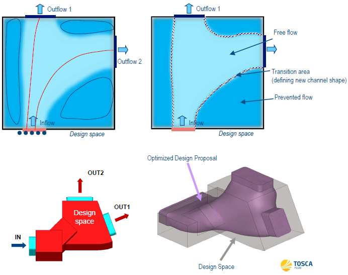
Excerpts from "CFD Topology and Shape Optimization of Ford Applications using Tosca Fluid" by Dr. Anselm Hopf, Ford Motor Company, Aachen, Germany: "The roots of Tosca Fluid have been developed at Daimler research in the early 2000s under the name AutoDuct (Klimetzek, 2006), (Moos, 2004)". One of its inventors, Dr. Klimetzek, explains the methodology of CFD topology optimization by looking to the nature of a river delta. Zones of backflow and recirculation have been eliminated by accumulation of sand, called sedimentation. Tosca Fluid is using the same bionic idea and thus called bionic optimization method. CFD topology optimization has been also implemented using mathematical adjoint methods (Othmer, 2006). Tosca Fluid has been implemented for STAR-CCM+ and ANSYS Fluent."
Optimization technology embedded in STAR-CCM+ is called STAR-Innovate which is an add-on license. Design Manager feature in STAR-CCM+ can create design exploration projects without needing any additional licenses. Design manager can be used for parameter sweep study exploring the design space that is combinations of parameters. STAR-CCM+ can be used with HEEDS technology for automatic intelligent search.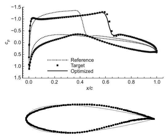
Morphing: In morphing technique, a new design variant is created as a complex combination of two or more objects which are geometrically different but topologically similar. Mesh morphing can be used for various purposes such as move onto a new known shape by just updating nodal positions, move onto a shape predicted by the CAE solution (shape optimization using adjoint solver) or move CFD wall boundary according to erosion/deposition.

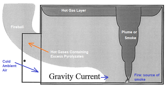
Fire modeling is partly modeling of a combustion phenomena. However, in contrast to a well-designed combustor, fire is random in nature. Still CFD simulations can be used to an accurate prediction for the spread of smoke and other toxic substances in the course of a fire.
Mathematical models for the simulation of fires depends on the use of zone models. These divide the compartment into two volumes in which the average properties are calculated as a function of time. With a zone model the fire room is divided into two distinct regions of gases, a hot layer towards the ceiling (which results from the hot buoyant gases arising from the fire forming a plume) and a cooler layer near the floor. When the plume reaches the ceiling it propagates along the ceiling, then slowly descends filling up the space. The height of this layer is dependent on the presence of openings into the compartment. The two regions of the zone model are treated as internally homogeneous control volumes for which the average properties are calculated by applying fundamental laws and correlations, as a function of time. For most situations that a fire engineer encounters, a zone model would provide an acceptable description of what would happen in the event of a fire.
Fire modeling using CFD methods (where the compartment or fire-room is split into many small cells or control volumes, within which conservation of mass, energy and momentum are enforced by applying the Navier-Stokes equations) is also called field modeling. One of the well known and thoroughly investigated phenomena in fire modeling is the "trench effect". It describes now a well established mechanism for fire propagation on enclosed slopes such as escalators or stairwells in building structures.
As observed during Kings Cross (London) Underground fire disaster in the 1987, studies into structural fires have revealed that the trench effect can produce extreme fire behaviour and rapid fire spread. Similarly, a wildfire will spread more rapidly up a slope than it will on flat terrain. The slope of the terrain brings the ground and hence the fuel upon it into closer proximity with the flames downstream the fire. This in turn extends the preheating range and allows for faster rates of spread.
Reference: Modelling Smoke Flow Using Computational Fluid Dynamics by TN Kardos, Fire Engineering Research Report 96/4, December 1996: "The phenomenon arises from a sudden entry of fresh air via a gravity current, into a closed space in which a fire has been burning. This space has accumulated an excess amount of fuel vapour, and with an ignition source results in a deflagration. the fuel can not be burned and will start to accumulate in the gaseous layer. This unburnt fuel is known as excess pyrolyzates. If a new ventilation source is introduced, such as a fire fighter opening a door or a window breaks due to thermal stress, the hot gases within the room flow out of the top of the vent and the cooler ambient air would flow in at the bottom.
The flow of cold ambient air into the room is known as the gravity current. The gravity current travels towards the ignition source through the bottom of the vent while hot gases containing excess pyrolyzates exit at the top. In the interface between the gravity current and the layer of hot gases from the leading edge or nose of the gravity current, and the region immediately behind the nose, mixing of the ambient air and excess pyrolyzates occurs.
As a result of mixing oxygen and the unburnt fuel, this region will tend to be within the flammable limits. When the gravity current reaches an ignition source the flammable mixture ignites and travels out along the interface of the gravity current and the layer of hot gases. The flow of gases behind the flame front is sufficiently turbulent to increase mixing in this area, this results in combustion in which the flame front travels below the speed of sound, termed turbulent deflagration, within the compartment. This combination of events helps to drive the excess pyrolyzates out of the compartment in an external fireball."
FDS: Fire Dynamics Simulator
As per "nist.gov/services-resources/software/fds-and-smokeview", FDS and Smokeview are free and open-source software tools provided by the National Institute of Standards and Technology (NIST) of the United States Department of Commerce. Fire Dynamics Simulator (FDS) is a computational fluid dynamics (CFD) model of fire-driven fluid flow. The software solves numerically a form of the Navier-Stokes equations appropriate for low-speed, thermally-driven flow, with an emphasis on smoke and heat transport from fires. CFAST: Consolidated Model of Fire and Smoke Transport, Smokeview (SMV) is a visualization program used to display the output of FDS and CFAST simulations.CGNS: CFD General Notation System which provides a general, portable and extensible standard for the storage and retrieval of computational fluid dynamics (CFD) analysis data. In other words, it is a standard for recording and recovering computer data associated with the numerical solution of the equations of fluid dynamics. CGNS facilitates the exchange of CFD data between sites, applications codes (software vendors) and across computing platforms and to stabilize the archiving of CFD data.
CGNS database comprise of:CFD Simulations for FE Engineers
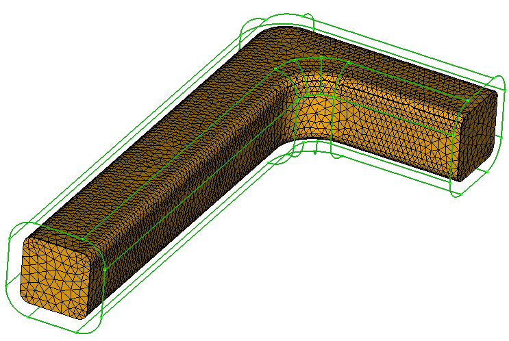
Most of the numerical simulations such as Finite Element Analysis (FEA) and Fluid Mechanics simulations such as CFD and CAA have lot of things in common. It is easy to participate in cross-application simulations activities if not to become a practicing analyst in both these disciplines. Following sections try to summarize the similarities and differences in FEA vs. CFD) approaches and activities.
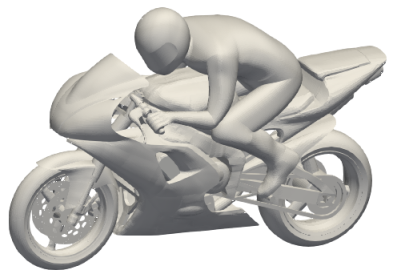
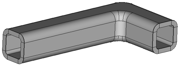
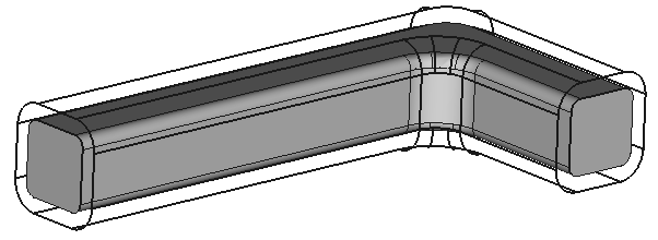
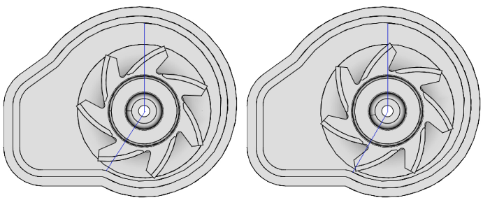
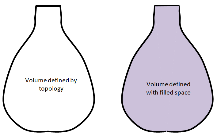
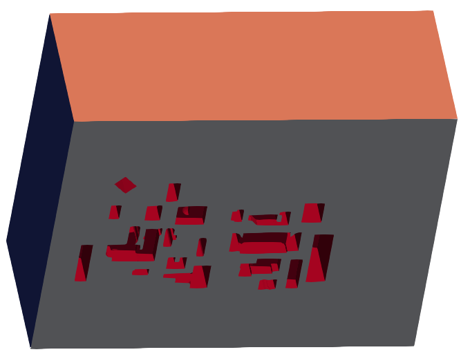
Can you describe what are the differences between two representations of the same 3D space?
Differences between FEA and CFD simulations
| S. No. | FEA | CFD |
| 01 | We model what we see! Let's call this as concept of modeling the "positive volume". | We usually model what we do NOT see. Let's call this approach as modeling the "negative volume". Note that there is nothing called a 'negative' volume. |
| 02 | Geometry Examples: CHT Domain: Q: what would be the simulation domain to model flow over this motor-bike with a rider? | FEA Domain:
|
| 03 | There is no concept of 'walls', 'inlet' and 'outlet' boundary conditions | The 'walls', 'inlet' and 'outlet' are the most basic ingredients of CFD simulations, there is no fluid without a 'wall' |
| 04 | FEA works on force and moment balance, calculation of displacement field which translates into strain and stress | CFD works on mass and energy balance, calculation of velocity and pressure fields which translate into pressure drops, viscous/shear forces and pressure forces on the walls |
| 05 | FEA cannot use hanging elements, it implies crack | CFD uses and even recommended sometimes to use hanging elements |
| 06 | FEA requires fine mesh near high stress gradient such as bends | CFD requires fine mesh near high velocity gradient such as walls |
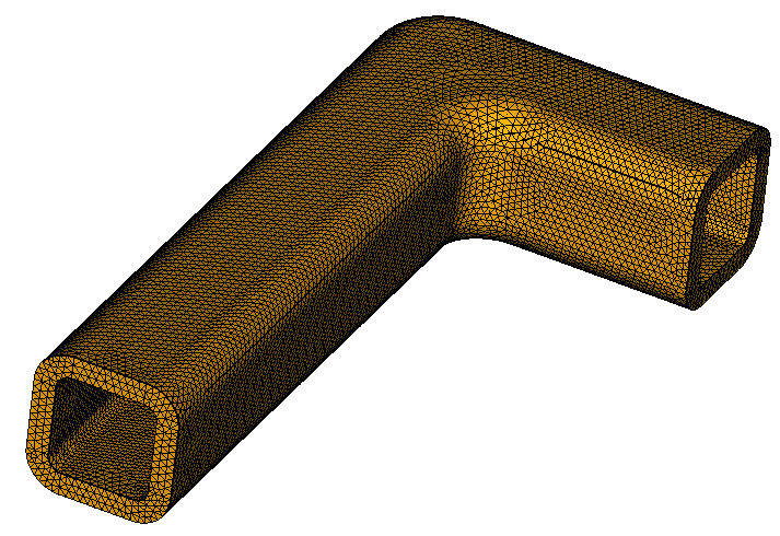
| 07 | Mesh Examples: the activity involves creating a closed volume - both for FEA and CFD mesh. Mesh of the FEA Domain:
| CAD geometry works on concept of edge, surface and volume. FEA / CFD pre-processor works on concept of topology and material points. Mesh of the CFD Domain: |
| 08 | FEA puts limit on mesh aspect ratio < 10 in most of the cases | CFD accepts aspect ratio up to 50 in cells or elements near the walls (called boundary layer or prism layer) |
Example of computational domain creation: the building planner is interested in knowing the flow pattern around the high-rise buildings. The information from simulation can be used for many purposes such as locating chimneys, gap between two adjacent towers to avoid humming noise...
Input: the 3D geometry of buildings
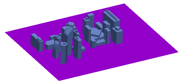
Computational domain - the space around the buildings
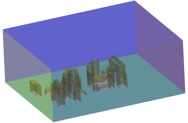
Computational domain - the solid model of buildings subtracted from the cuboid
Similarities between FEA and CFD simulations
| S. No. | Description | Remark |
| 01 | Both applications uses all types of elements: tri, quad, tetra, wedge / prism, hexahedrons | There is no concept of higher order elements in CFD |
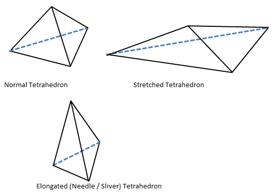
| 02 | Same pre-processor can be used to generate mesh for FEA and CFD. | Boundary layer mesh generation is nothing but a finer mesh near the walls. Why wedge (prism) and hexahedron elements are used in boundary layer and not tetrahedrons? The answer lies in definition of aspect ratio and tetra-collapse? |
| 03 | Both conformal and non-conformal contacts can be used in FEA and CFD. | In CFD, it is known as 'interfaces'. Since the number of interfaces can be very high in CFD, it is normally recommended to keep less number of interfaces or avoid altogether. |
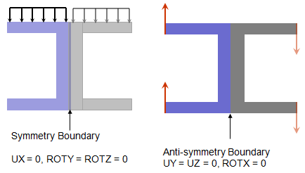
| 04 | Periodicity and symmetry / anti-symmetry | FEA uses symmetry but does not use concept of periodicity. CFD simulations do not use concept of anti-symmetry. |
| 05 | Most FEA and CFD programs can solve thermal conduction phenomena without modeling the fluid flow if temperature and other heat transfer boundary conditions are known. | In FEA, it is used to find thermal stress. In CFD, it is used to make a quick calculation of hot spot temperatures. |
Tetra-Collapse: The height of the Tetra element is measured from each of the four nodes to its opposite face and then divided by the square root of the area of opposite face. The minimum of four resulting values is then normalized by dividing it by 1.24. As the size of tetrahedron collapses, the value approaches to 0. While a perfect tetrahedron has a value of 1.0, tetra-collapse values < 0.2 are generally not acceptable in most of the simulations.
The exchange of information between FEA and CFD engineers can be in terms of topology checks and mesh quality parameters required for FLUENT Mesher and STAR-CCM+
| S. No. | Description | Checkpoint | Actual value in the mesh |
| 01 | Mesh Type | Surface mesh, all tri-elements | - |
| 02 | Minimum size | 2.0 [mm] | - |
| 03 | Maximum size | 16 [mm] | - |
| 04 | Total 2D cell count | 2,00,000 | - |
| 05 | Topology: number of free edges | 0 | - |
| 06 | Topology: number of self-intersections | 0 | - |
| 07 | Topology: number of penetrating elements | 0 | - |
| 08 | Topology: number of duplicate elements | 0 | - |
| 09 | Topology: number of over-lapping elements | 0 | - |
| 10 | Quality: skewness [0 is ideal, 1 is degenerate] | ≤0.60 | - |
| 11 | Quality: aspect ratio | ≤5.0 | - |
| 12 | Quality: surface deviation* | ≤0.1 [mm] | - |
| 13 | PID / Zone naming | as per naming convention agreed upon | - |
The engineering services has grown to the extent that a new category of companies ESP (Engineer Service Providers) has come into vogue. These companies supplement the resources (work-forces, hardware, software) to brand owners known as OEM (Original Equipment Manufacturers).
Why companies outsource the simulation tasks?What to do when CFD simulations take more time and cost more than developing a prototype and carrying out actual tests
The short answer is: "Do not use CFD simulations unless you want to integrate it into product development cycle". A detailed answer is: If the company or team has strong knowledge management systems and methods/principles of product design are well established, CFD simulation may seem an overhead initially. How do you known what to improve if your product does not meet specification in first prototype? How many iterations are typically needed to meet those specifications through "Redesign -> Develop Prototype -> Test -> Redesign" loop? The advantage of virtual simulations is that they provide vast amount of data and an appropriate investigation helps immensely in root-cause analysis.Evaluation and Comparison of CFD Simulation Tools
The pricing structure of modern CFD tools are getting modular. There are three distinct category of licenses: Pre-Post, Solver and Parallel operation (known as HPC: High Performance Computing). A type of license which packs all 3 features in one is sometimes call a 'Bundled' license. They are designated differently such as Standard, Perpetual, Leased or Term License, Student Version, Academic, Professional, Suite, Power, Premium, Network License, Batch License, Floating License (WAN-type, LAN-type, Global), On-Demand, Enterprise, Node-locked or CPU-Locked, User-locked or Named Single-user License, Credits-based or Tokens-based, Add-on... Most of commercial tools have mix of licenses: For example, STAR-CCM+ Lite license does not allow to set-up a case with thermal radiation, multiphase, SMM and Coupled solver. Seats or ccmpsuite (serial) license of STAR-CCM+ allows to open a session of STAR-CCM+ on one core. Additional 'seats' can be used as additional cores. Parallel processing or HPC licenses are known as power tokens in STAR.
ANSA uses credit based license system where with 100 credits one user per computer can open simultaneously as many ANSA sessions as they want. ANSYS FLUENT requires HPC Packs to make simulations in parallel with number of cores more than 4. However, one thing which is often missed is the tools required to clean-up and defeature the simulation geometry. The comparison of two CFD codes needs to be done on mainly 5 factors:
| Geometry Clean-up | Pre-Processing (Meshing) | Pre-Processing (Solve Set-up) | Separate HPC? | Post-Processing |
| ANSA | ANSA | FLUENT | Y | FLUENT |
| ANSA | FLUENT | FLUENT | Y | Tecplot |
| STAR-CCM+ | STAR-CCM+ | STAR-CCM+ | N | STAR-CCM+ |
| SpaceClaim | ANSA | FLUENT | Y | FLUENT |
| SpaceClaim | HyperMesh | STAR-CCM+ | N | STAR-CCM+ |
Similar way, the features of software also need to be compared such as:
Note that as on V2022, ANSYS ICEPAK needs the mesh to be generated inside ICEPAK environment. STAR-CCM+ has a Power license option which provides unlimited parallel operations. ANSYS FLUENT provides modular HPC Packs where you add a module as you ramp-up the parallel operations. All these options point to the fact that the cost-effectiveness of any particular set of tools as tabulated above shall depend on the number of users. For small number of users, modular licensing may not help. On the other hand, as the number of users increases significantly, modular structure of licenses may turn out to be more effective. Other factor which needs to be considered is the available HPC hardware. If the solver runs are limited to fewer number of cores, a modular licensing may be beneficial.
A precise definition of any "technical issue" is 50% of its resolution. An important aspect to remember is ability to distinguish 'cause' and 'effect' where one tends to swap the two.
Effect: Water started boiling, Cause: Water was heated and the molecules started moving quickly.
Effect: The ocean have tides, Cause: The moon creates gravitational pull.
Effect: Sales is in downtrend, Cause: There is no new order and/or delay in ongoing projects.
The cause-and-effect discussion can be organized in one of these two primary ways:
CFD Simulations in Various Phases of Product Development Cycle
Preliminary Design Review (PDR) is performed during the Design and Engineering Phase when the System Developers create a baseline high-level system architecture with a reasonable expectation of satisfying the requirements. This phase of development does not require any simulations activities and are mostly based on past experiences and domain knowledge. A PDR is conducted before the start of detailed design work.
Preliminary Design Review (PDR) is conducted to ensure new technologies are mature enough to be integrated into a product subsystem to form its allocated baseline. A Critical Design Review (CDR) is focused on determining if a system can meet its stated performance requirements within cost, schedule, and risk. CDR is the phase when numerical simulations may need to be performed to get some baseline insight into the hydraulic and thermal performances.
Assumptions in Flow and Thermal Simulations
CFD simulation documentation should consists of Scope, Computational Domain, Boundary Conditions, Material Properties, Mesh Type and Solver Settings, Methodology, Assumptions, Acceptance Criteria and Deliverables.| S. No. | Description of Assumption | Justification and impact on accuracy of result |
| 01 | Material properties shall be assumed constant | Not function of temperature except when air is modeled as Ideal Gas |
| 02 | All walls shall be assumed hydraulically smooth | Most of the time boundary layer thickness exceeds the roughness height |
| 03 | ... | ... |
| 04 | Thermally perfect contact between two solid surfaces | Contact resistance can be modeled if known |
| 05 | Polyhedral mesh, k-ε turbulence model with target wall 30 ≤ y+ ≤ 100 | k-ω turbulence model with target wall y+ ≤ 1 shall require separate budget |
| 06 | ... | ... |
| 07 | Geometry to be defeatured by removing fillets and chamfers ≤1 mm | A compromise between accuracy of geometry and accuracy of mesh |
| 08 | If geometry contains fins, geometry with only plane walls considered | Thin sections with wavy surfaces or holes or dimples require very fine mesh, separate timeline and budget shall be shared |
| 09 | No swirl applied for fan boundary condition: flow 100% axial | Tool has capability to model swirl, recommended 10% |
| 10 | ... | ... |
| 11 | Turbulence at inlet modeled as Turbulent Intensity, TI = 5 and Turbulent Viscosity Ratio, TVR = 10 | Should be reduced to TI = 1 and TVR = 2 if flow is coming out of a straightener |
| 12 | Uniform flow assumed at inlet (no parabolic or 7th power profile) | Extend domain [50 x Hydraulic Diameter] if fully developed flow is expected |
| 13 | Only surface mesh and case file shall be stored for 2 years | Surface mesh contains all settings to generate volume mesh |
| 14 | Volume mesh and result files shall not be stored | Case file contains volume mesh data |
| 15 | Single precision solver shall be used | It is reasonably accurate and saves computational memory. |
The word system is a self-enhancing or self-growing concept. The dictionary meaning of a system is "a regularly interacting or interdependent group of items forming a unified whole". In an automotive system, there is a term called "Seating System" which refers to the seat, recliner mechanism, seat belt anchor... However, in context of full car, it is just a sub-sub-system. Similarly, in case of a data centre, everything inside the roof or even devices put on the roof and below the floor may comprise of a system. Though for the sake of evaluation and modularity, the racks, the plenum and ducts, computer room air conditioning (CRAC) and computer room air handler (CRAH)... can be considered independent systems.
| Number of different geometries: | [ - ], nGEO | |
| Number of boundary conditions per geometry: | [ - ], nBC | |
| Effort to generate mesh per geometry1: | [hours], tMSH | |
| Effort to set-up a baseline case2: | [hours], tSOL | |
| Effort to set-up an iteration case2: | [hours], tITR | |
| Time to upload set-up file, download result file: | [minutes], tDAT | |
| Number of contour plots per case: | [ - ], nPLT | |
| Number of quantitative data per case: | [ - ], nQ | |
| Number of graphs to be generated per case: | [ - ], nC | |
| Time taken to generate one plot*: | [minutes], tP | |
| Time taken to extract data and generate graph: | [minutes], tC | |
| Time taken to insert 6 images on a slide and arrange: | [minutes], tS | |
| Time to load one result file for post-processing: | [minutes], tL | |
| Calculate project duration (human efforts) | ||
Installation and Licensing
Each program has different installation and license configuration methods. For ANSYS suite of products, the video on YouTube.com titled "Installing ANSYS 2023 Releases on Windows" explains the method. As per the instruction, user has options to select the product(s) to be installed. The video titled "Licensing Settings Utility Configuration" explains step-by-step method for configuring license servers.

For ANSYS Electronic Desktop, license server specification may also be done inside the ansyslmd.ini file (create a file if does not already exist). File content is: SERVER=1055@lic_server_name where the name or the IP address of the machine that runs the ANSYS License Manager is lic_server_name. The flexnet port 1055 is the default which can be changed by administrator. Alternatively, license server specification can be done with environment variable ANSYSLMD_LICENSE_FILE = 1055@lic_server_name. The variable supersedes the ansyslmd.ini file.
License Manager needs to be installed on the Windows machine that will act as a license server. It is not necessary to install the Ansys License Manager on the "client" computers.
How to install ANSYS AEDT: support.ozeninc.com/ help-center/ how-to-download-and-install-ansys-electronics-desktopTable of Contents
Similarities between FEA and CFD simulations |=| System Modeling [*] Step-by-Step Guide to CFD Simulation {*} Convergence and relaxation factors ]=[ Reduced Order Modeling (*) Fluid Network Method [/\] SU2: Stanford University Unstructured [\/] DOE in CFD Simulations {/} Adjoint Solvers [=] CGNS: CFD General Notation System (=) Assumptions in Flow and Thermal Simulations {=} Erosion Modeling /=/ Outsourcing of CFD Simulations: Why and When? /=/ Example problems in Fluid Mechanics and Heat Transfer /=/ Wind Turbines /=/ Metro Route Finder /=/ Octave Scripting /=/ Computer Vision /=/ Web Technology /=/ Stock Market /=/ Electronic Cooling /=/ Job Description Template /=/ जीवन के महत्वपूर्ण अनुभव - Lessons of Life /=/ जल का संरक्षण - Rainwater HarvestingPublish your article or get a backlink from this website: In case you want to publish any article on this website with your name and contact details or get a backlink to any specific section of your own website, please write to the email address given in footer section.
Step-by-step approach to CFD simulations using commercial tool ANSYS CFX / FLUENT or open-source product like OpenFOAM, textbook solutions to Fluid Mechanics problem, quiz on CFD and FEA are covered on this site. Various physics like simulations of multiphase flows, rotating machines are covered with examples. The content on CFDyna.com is being constantly refined and improvised with on-the-job experience, testing and training. Examples might be simplified to improve insight into the physics and basic understanding. Linked pages, articles, references, and examples are constantly reviewed to reduce errors, but we cannot warrant full correctness of all content.
Template by OS Templates
 Visit the blog page to view topics on mathematics, human resource, textbook solutions, data analytics in stock market trading, online quizzes and much more ...